Karl Ho
School of Economic, Political and Policy Sciences
University of Texas at Dallas
A New Generation of
Data Storytelling
Prepared for Love Data Week, Office of Research and Innovations, University of Texas at Dallas, 2/14/2024
-
Karl Ho is:
- Professor of Instruction at University of Texas at Dallas (UTD) School of Economic, Political and Policy Sciences (EPPS)
- Co-founder of the UTD Social Data Analytics and Research program (SDAR)
- Course: EPPS 6356 Data Visualization
- Founder of DataGeneration.io
- Author of Data Programming
- Principal Investigator of the Taiwan Studies Project in UTD
- Co-Principal Investigator of the Hong Kong Election Study project
- Website: karlho.com (talks, lecture, publications)
Speaker bio.
This presentation introduces the new generation of data storytelling: how to let data more effectively bring home the message and guide us to identify problems and better solutions. When we design and visualize the data, we will observe basic principles but more importantly, how can we make it future proof?
Overview:
In other words, we want to scale data visualization for:
-
Future self and new collaborators
-
Newer data
-
More complex setup and models
-
More user friendliness
What is data visualization?
What is data visualization?
-
Data visualization is to deliver a message from your data.
-
It is like telling a story using the chart or data applications.
-
Sometimes the data is huge or the story to too long to tell.
-
Visualization provides an ability to comprehend huge amounts of data. The important information from more than a million measurements is immediately available.
What is data visualization?
Data visualization is to communicate data patterns, findings and insights via visual representation of data. It is well beyond just creating a chart but to train "Thinking Eyes" and build data literacy.
Data: Daily COVID deaths
Dashboard: Live data
Dashboard: Live data
Dashboard: Live data
What is data visualization?
-
Learn to read your data
- Visual thinking
- Educated eyes
Wickham
A grammar of graphics is a tool that enables concise description of the components of a graphic.
Such a grammar allows moving beyond named graphics and gain insight into the deep structure that underlies statistical graphics.
Wilkinson
A grammar is a formal system of rules for generating lawful statements in a language.
The grammar of graphics goes beyond a limited set of charts (words) to an unlimited world of graphical forms (statements).
The rules of graphics grammar are sometimes mathematical and sometimes aesthetic.
Data Storytelling
-
If Data visualization is to deliver a message .....
-
Data storytelling is to give the whole picture.
-
It is the single hub that exhibits the issues or problems, and prescribes the solutions!
-
It goes beyond giving one chart!
-
One needs a Data Storytelling Station.
From data visualization to data storytelling
Next generation must be .....
-
Scalable
-
Reproducible
-
What if's
Scalable
-
Prototyping with design
-
Ready for bigger team
-
Future ready (readable by the future you)

Photo credit: Shane Rounce on Unsplash
Reproducible
-
Notebook based
-
Frequent editing
-
Ready to deploy
Photo credit: Nagara Oyodoon Unsplash

What if's - User input
Photo credit: Tim Mossholder on Unsplash

New tools: Quarto
What is Quarto?
- Quarto provides a unified authoring framework for data science, combining your code, its results, and your prose.
- Quarto documents are fully reproducible and support dozens of output formats, like PDFs, Word files, presentations, and more.
- Hadley Wickham
New tools: Quarto
What is Quarto?
- Quarto is Markdown and notebook-based. It allows generation of code-embedded documents readily convertible to websites, LaTeX, books and presentations.
- Quarto websites can be portable to GitHub for free-hosting!
- E.g. karlho.com, karlho.github.io
Shiny for Python applications
New tools: Shiny
What is Shiny?
- Shiny is a suite of tools to facilitate building of interactive web apps.
- Shiny is multilingual: R, Python and Observable (JavaScript)
- Features:
- Reactivity (user inputs)
- Interactive with js and wasm.
-
Most browsers intrepret html, xml, etc.
-
Visualization or fancy interactive charts are JavaScript (e.g. Plotly, D3)
-
The new language browsers speak is wasm (Wa-some)
New Technology to make this happen: WebAssembly or wasm.
-
emscripten
-
Pyodide: Python stack (NumPy, Matplotlib, and Pandas)
-
Shiny running on Pyodide: Shinylive.
-
WebR
WebAssembly or wasm.
\(\because\) Shiny is written in R
\(\because\) R is written in C++
\(\because\) can be compiled to wasm
\(\rightarrow\) \(\therefore\) Shiny can be compiled to WASM.
WebAssembly or wasm.
Serverless Shiny with Shinylive

Source: Joe Cheng "Running Shiny without a server"
Shiny for Python (ready to deploy)
Shiny for R (ready to deploy)
Shinylive applications
Source: Rami Krispin GitHub
Social media
Summary
Data visualization is evolving fast.
It must move from creating charts to giving storytelling dashboards.
It must be scalable, reproducible and reactive (allowing users to generate data in different scenarios).
This demonstration provides the latest development of the technologies and data storytelling design.
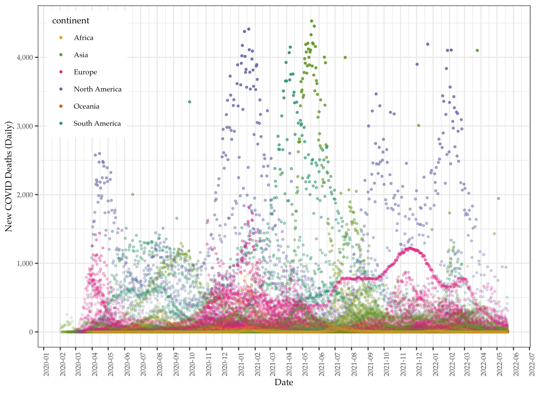
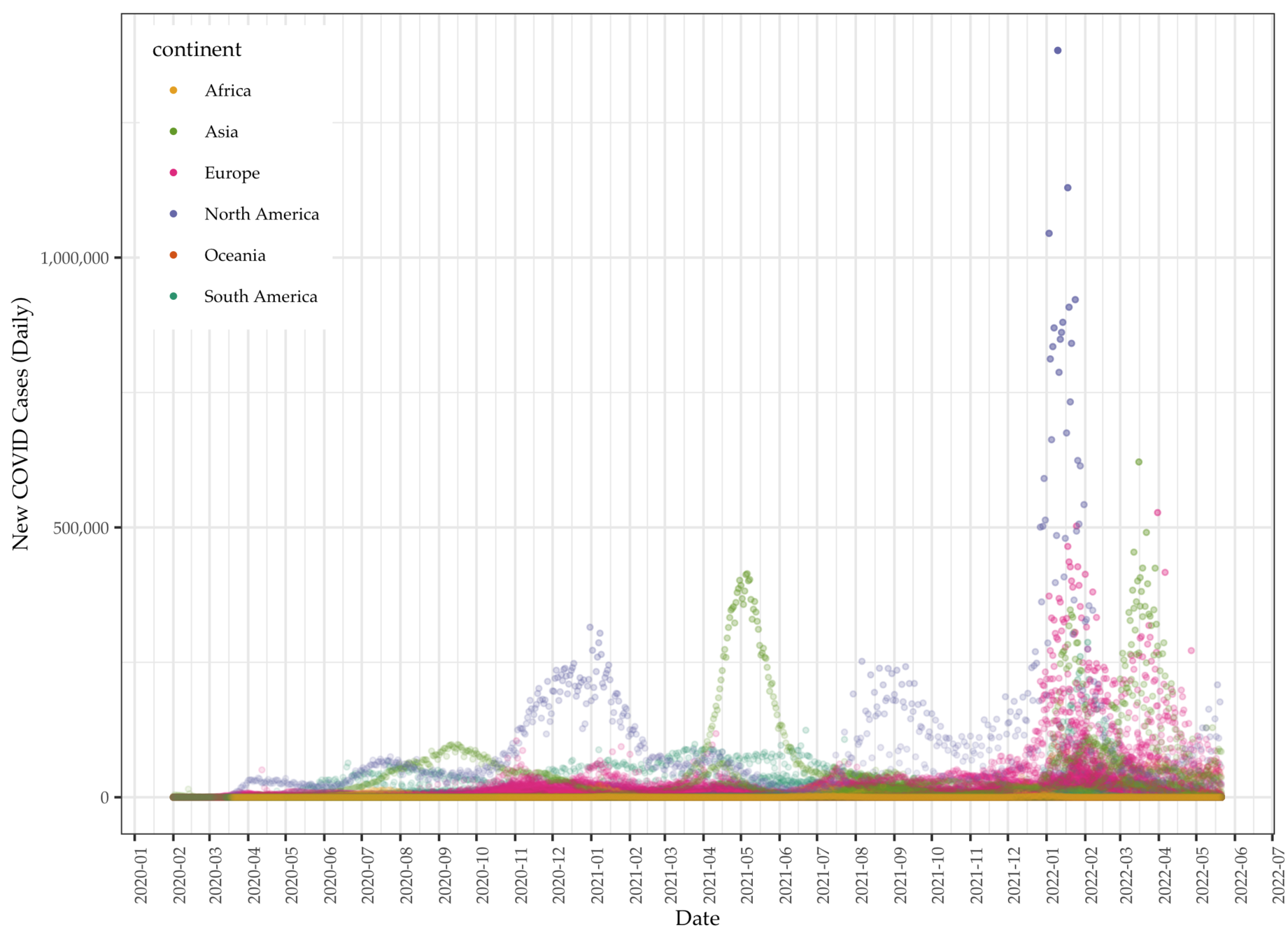
We collect global COVID data from the Our World in Data project, which makes available daily pandemic data from all countries available in real time.
- The data set comes with a series of daily variables (individual) including total (cumulative) and new cases (per million), deaths (per thousand), vaccination, and other longer-term variables (aggregate) such as GDP per capita, proportion of aged 65 or above, human development index (HDI), etc.
- There are a total of 225 units, with 212,580 cases (as of late October, 2022) and 67 variables.
- We use the peak-day data for modeling, which is on 1/20/2022. On that day, the United States having most COVID cases among all countries the recorded a cumulated 97,410,671 cases.
Illustration: COVID data
Data: Daily COVID deaths
Data

Data
- We focus on aggregate instead of daily data to identify predictors of total cases of COVID (per million).
- COVID data vary tremendously over countries and time. Singling out cumulative or total cases to regress on country-level variables allows modeling the COVID data per individual countries' characteristics
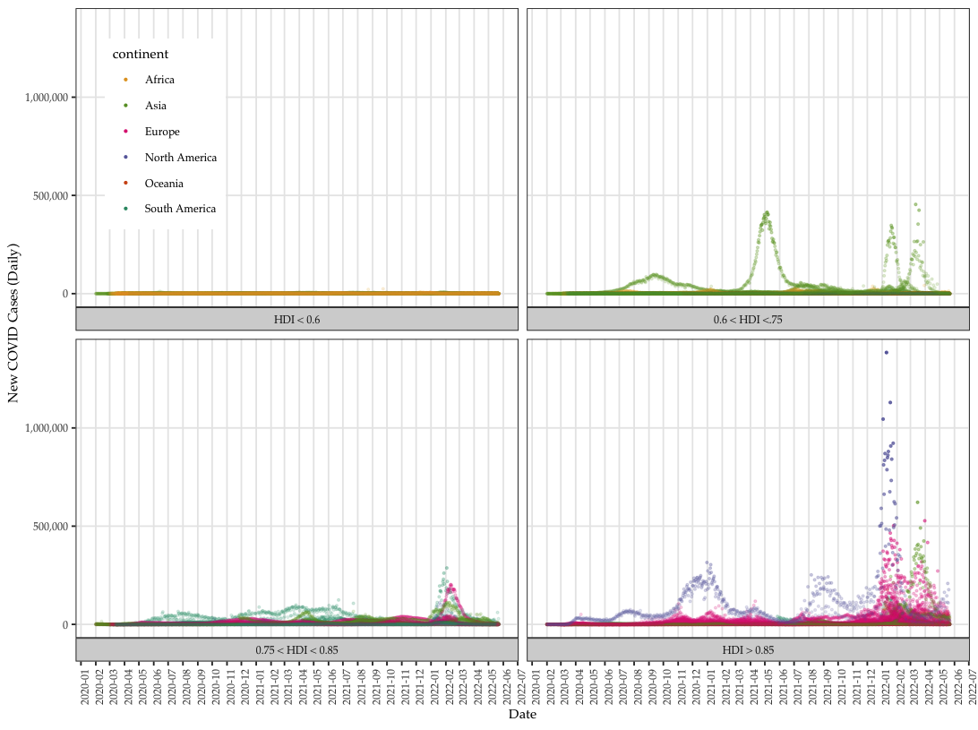
- OWID data point to one direction: how developed the country is and the number of COVID cases and death.
- The general trend is the more developed the countries are the more affected by COVID.
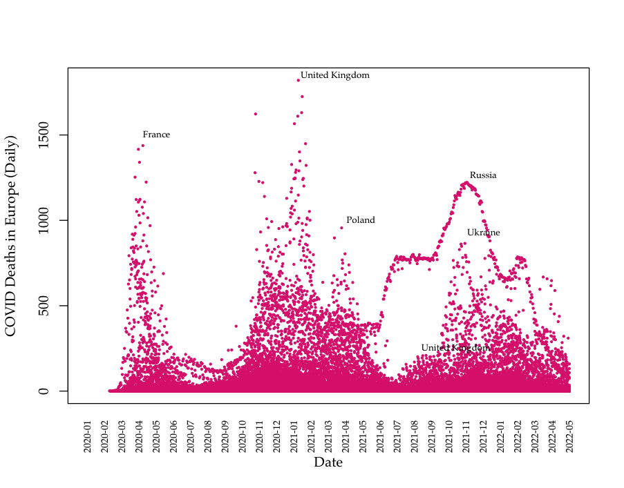
Data: Death data (Europe)
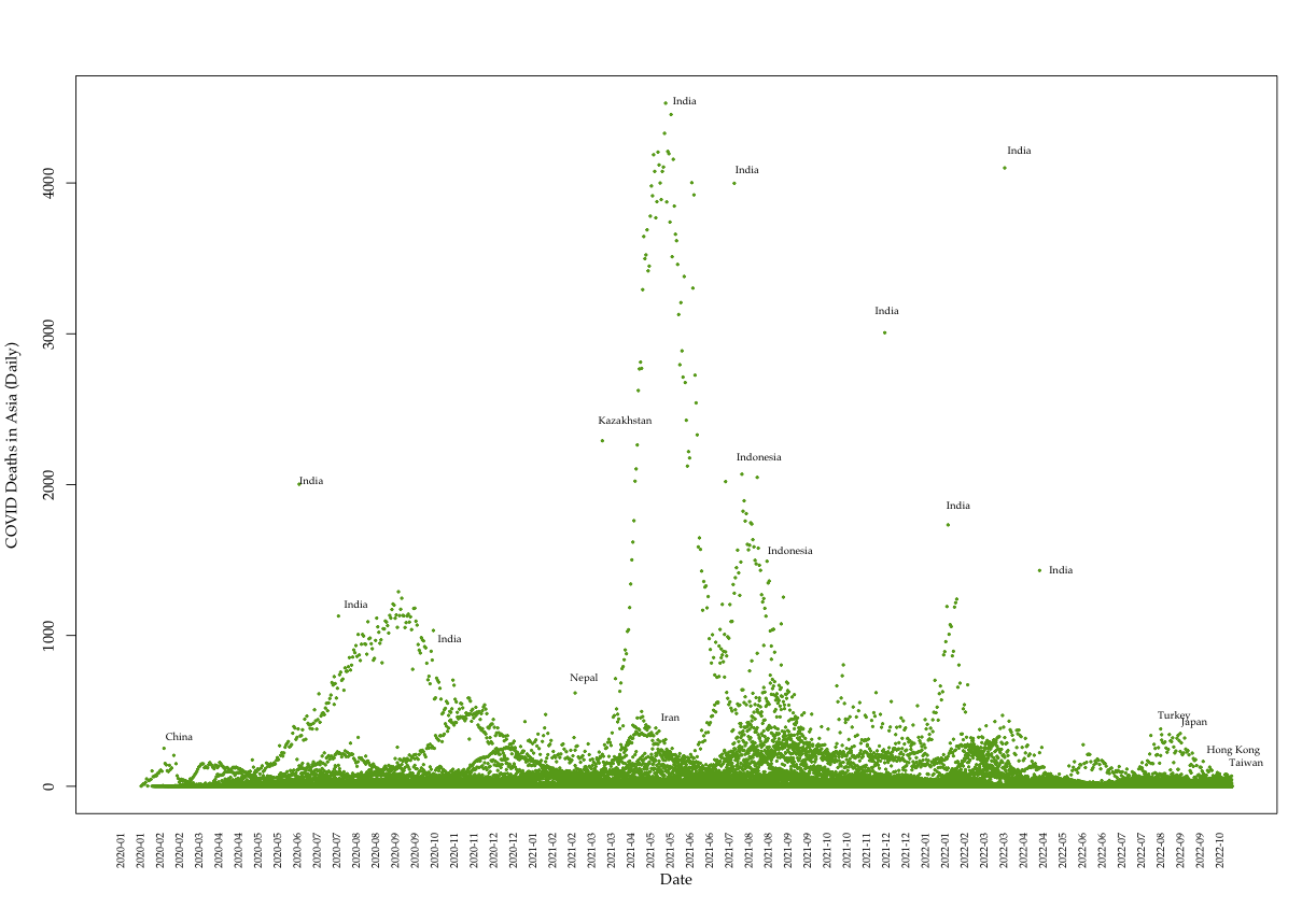
Data: Death data (Asia)
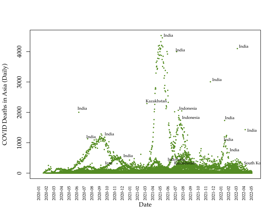
Most recent Data: Deaths (Asia)
Automated Machine Learning
- Automated machine learning applies multiple algorithms and modeling methods including:
- validation
- training and testing data partitioning
- pruning for tree models
- constraints application
- The process compares model efficacy using a series of metrics to determine stopping and selection recommendations including MSE, AUC and RMSE.
- We use \(H_2O.ai\) to model the COVID cases with 13 predictors.
Automated Machine Learning
Automated Machine Learning

Automated Machine Learning
COVID data using isoreg classification
Data: Total cases per million
Data: Daily COVID deaths
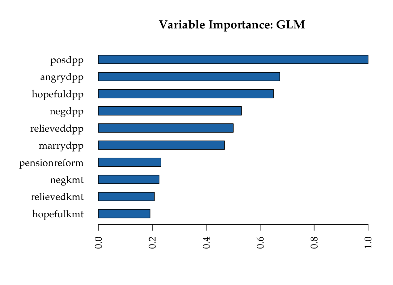
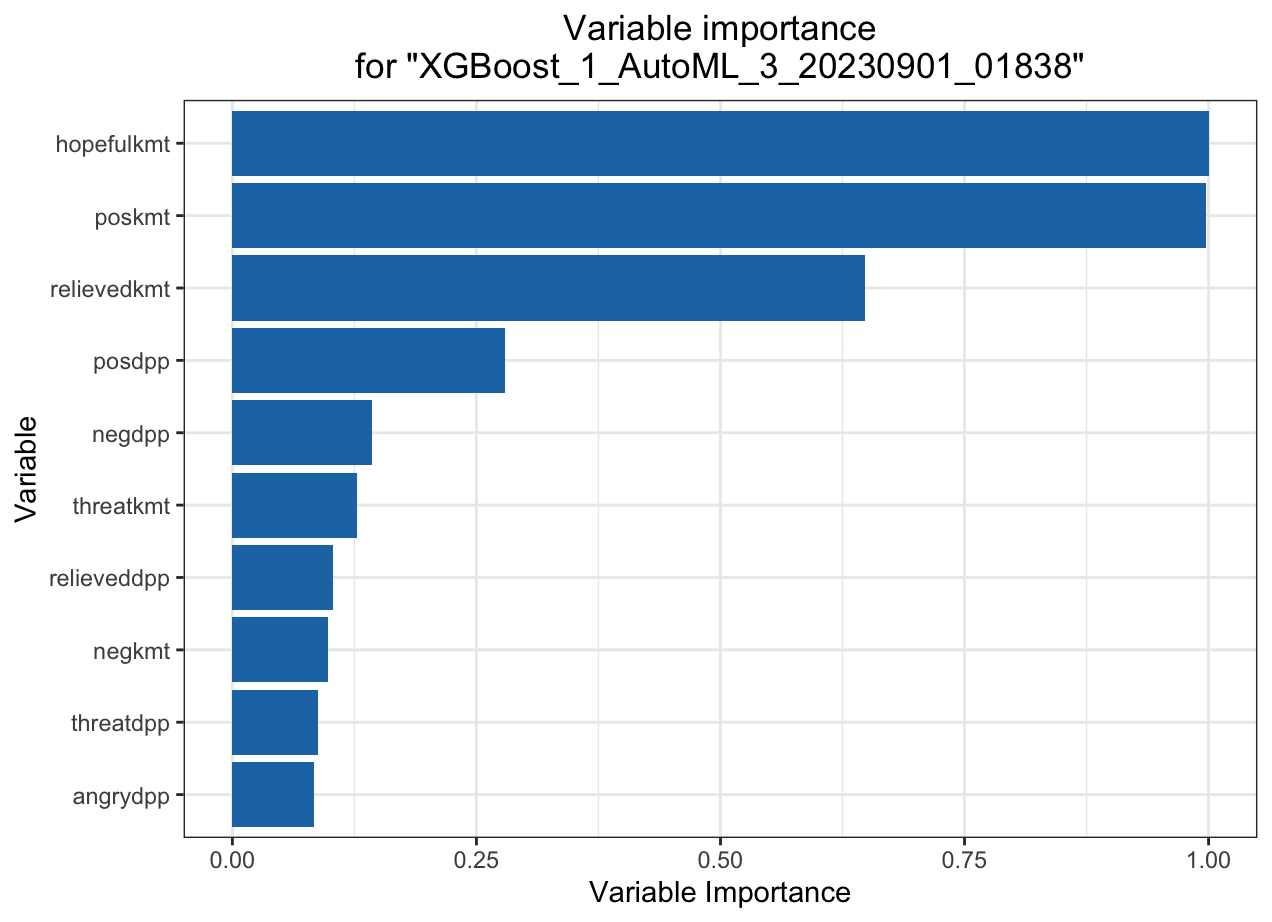
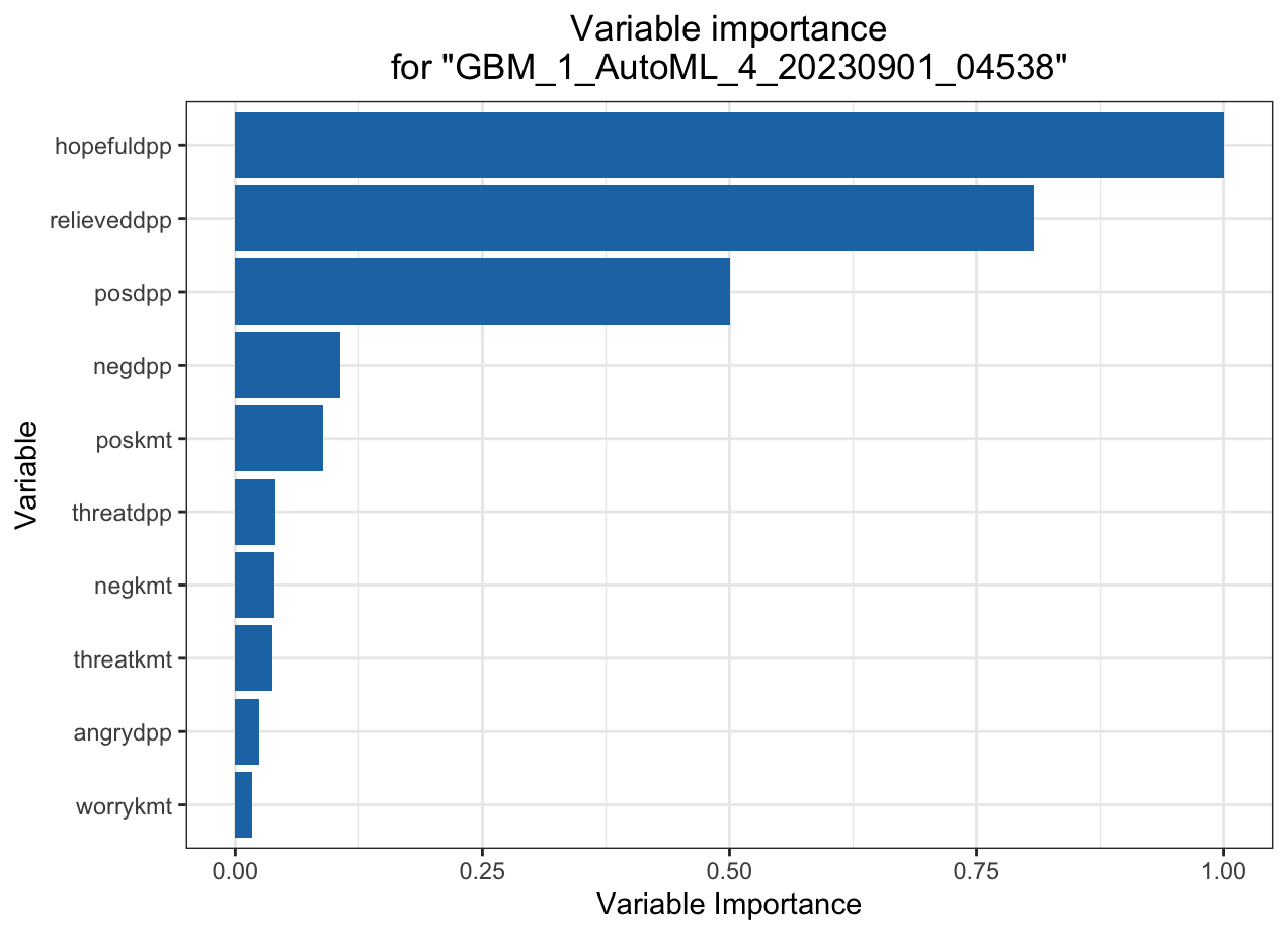
Most important variables: GLM
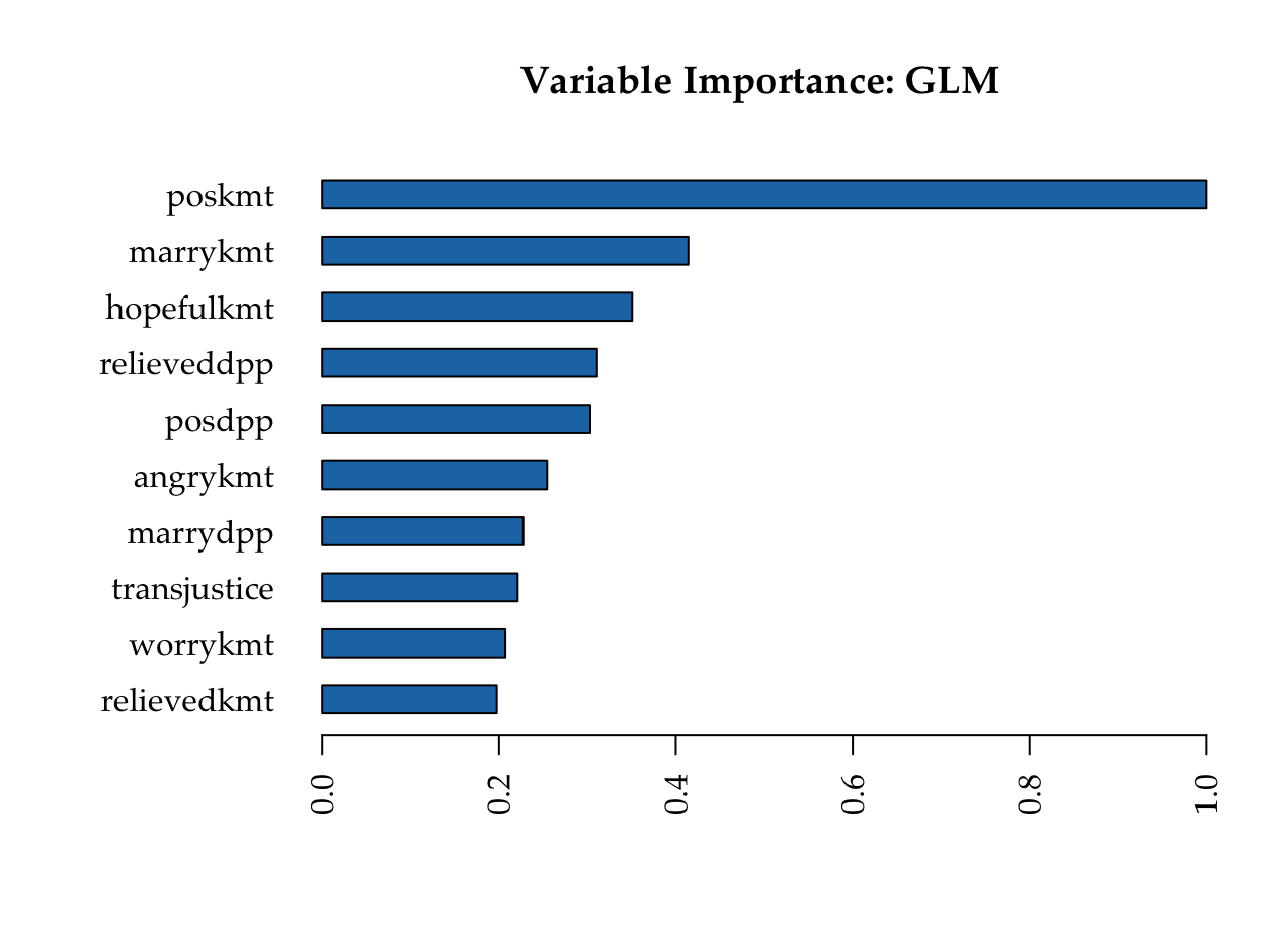
KMT
DPP
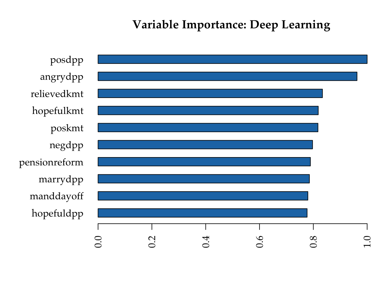
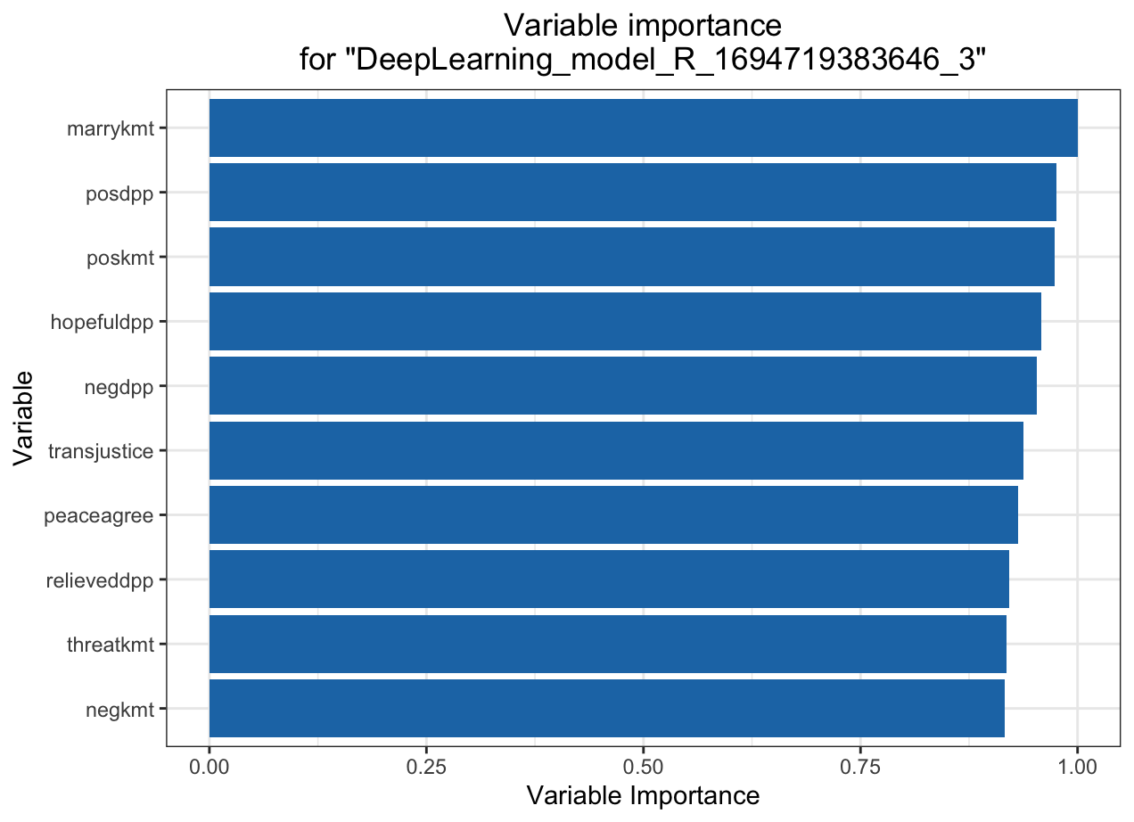
Deep learning model (NN)
KMT
DPP
MSE: 0.05650798
RMSE: 0.2377141
LogLoss: 0.190111
Mean Per-Class Error: 0.07756352
AUC: 0.9773588
AUCPR: 0.9645369
Gini: 0.9547177
MSE: 0.05053361
RMSE: 0.2247968
LogLoss: 0.1659664
Mean Per-Class Error: 0.08273317 AUC: 0.9781768
AUCPR: 0.9399842
Gini: 0.9563536
Automated Machine Learning: KMT
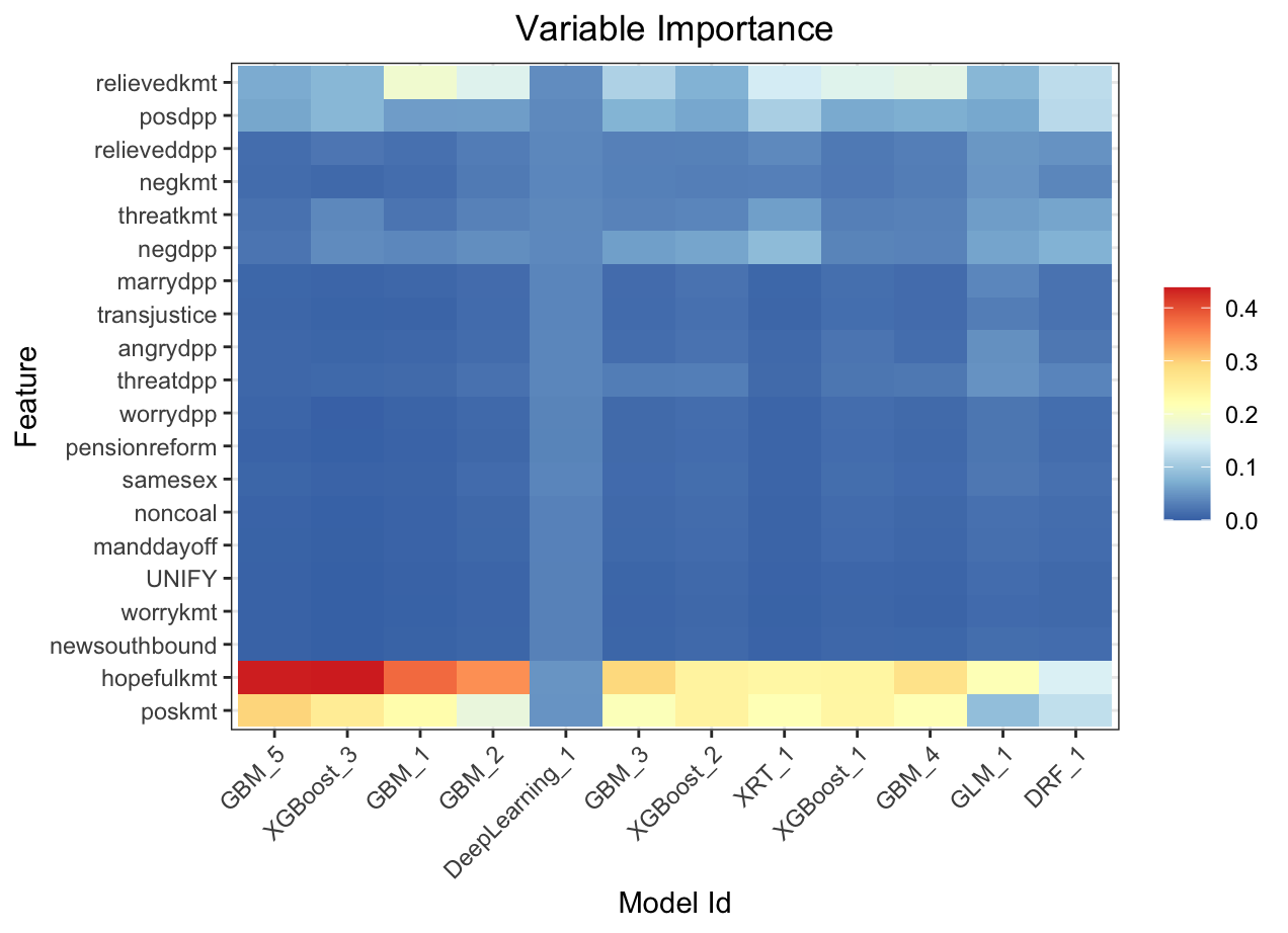
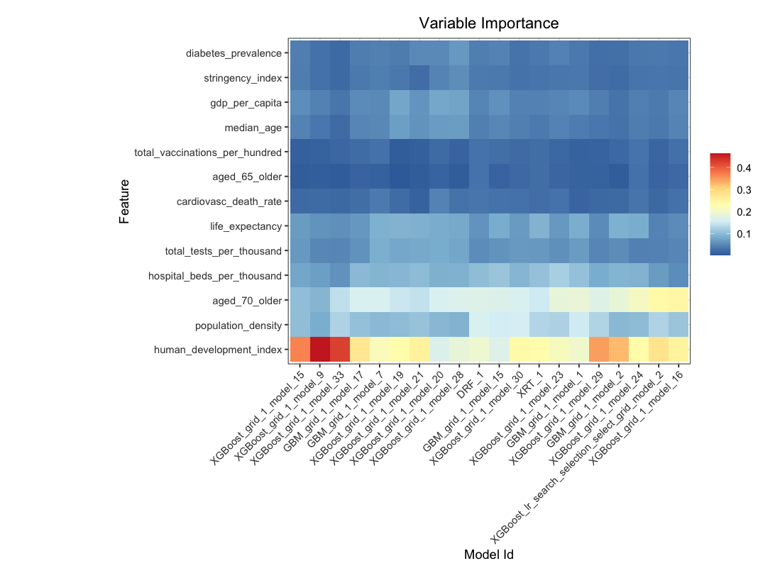
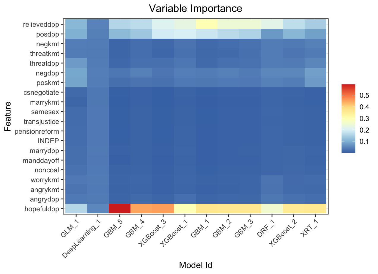
Variable importance heatmap shows variable importance across multiple models. Some models return variable importance for one-hot (binary indicator) encoded versions of categorical columns (e.g. Deep Learning, XGBoost). In order for the variable importance of categorical columns to be compared across all model types we compute a summarization of the the variable importance across all one-hot encoded features and return a single variable importance for the original categorical feature. By default, the models and variables are ordered by their similarity.
Automated Machine Learning: KMT
Variable importance heatmap shows variable importance across multiple models. Some models return variable importance for one-hot (binary indicator) encoded versions of categorical columns (e.g. Deep Learning, XGBoost). In order for the variable importance of categorical columns to be compared across all model types we compute a summarization of the the variable importance across all one-hot encoded features and return a single variable importance for the original categorical feature. By default, the models and variables are ordered by their similarity.
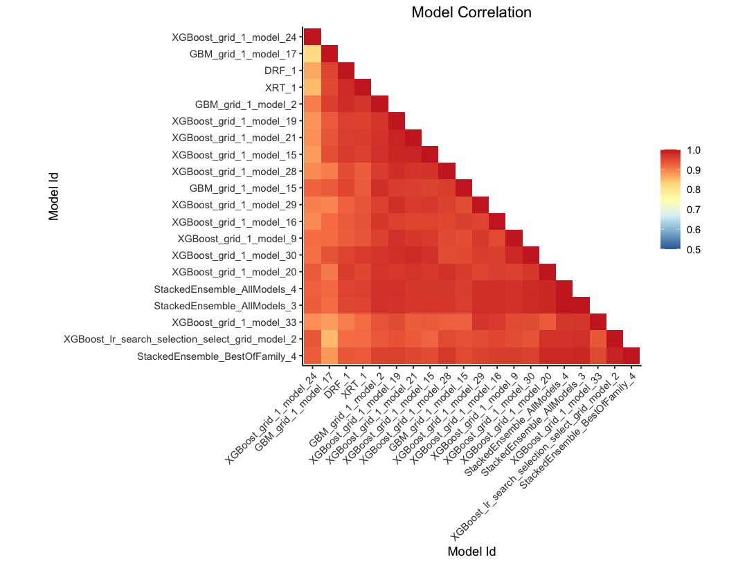
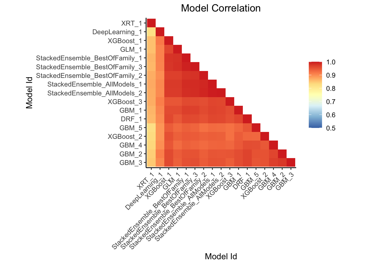
This plot shows the correlation between the predictions of the models. For classification, frequency of identical predictions is used. By default, models are ordered by their similarity (as computed by hierarchical clustering).
Automated Machine Learning: KMT
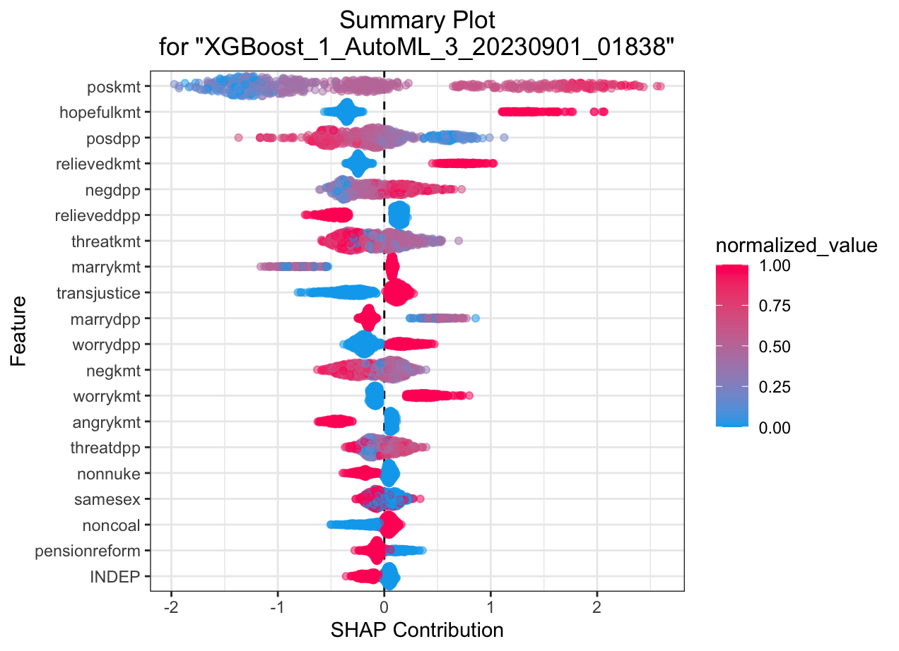
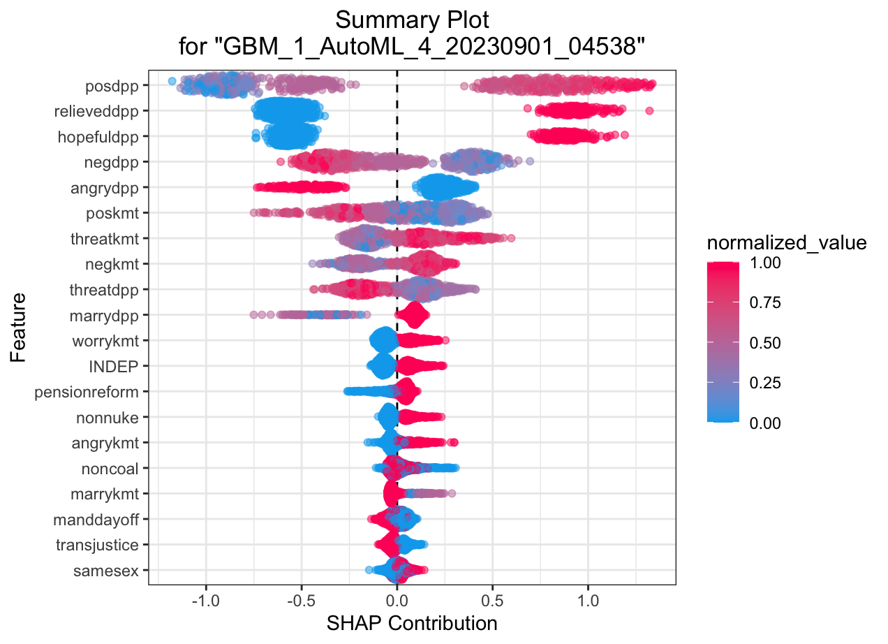
SHAP summary plot shows the contribution of the features for each instance (row of data). The sum of the feature contributions and the bias term is equal to the raw prediction of the model, i.e., prediction before applying inverse link function
Automated Machine Learning: KMT
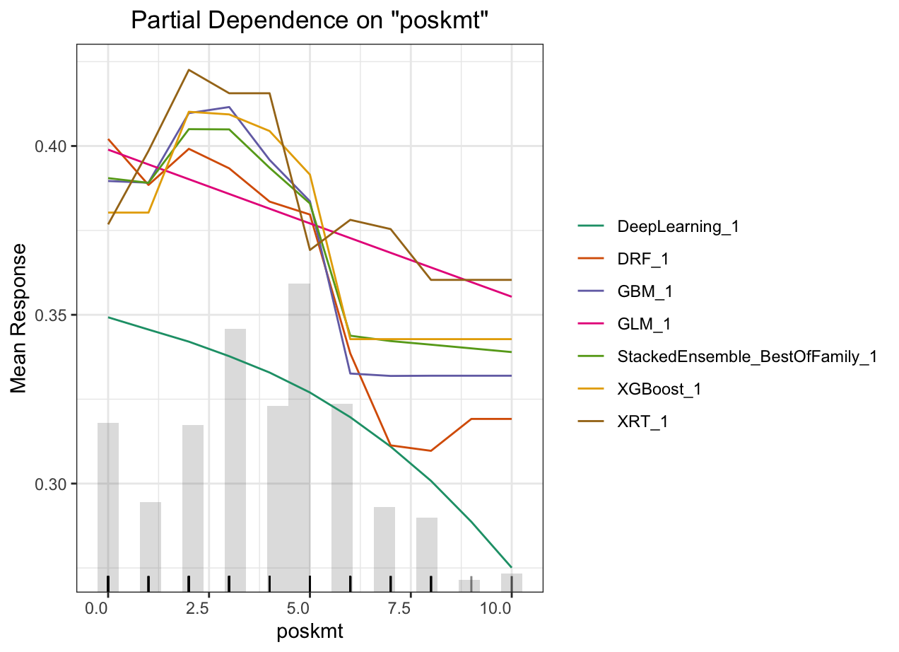
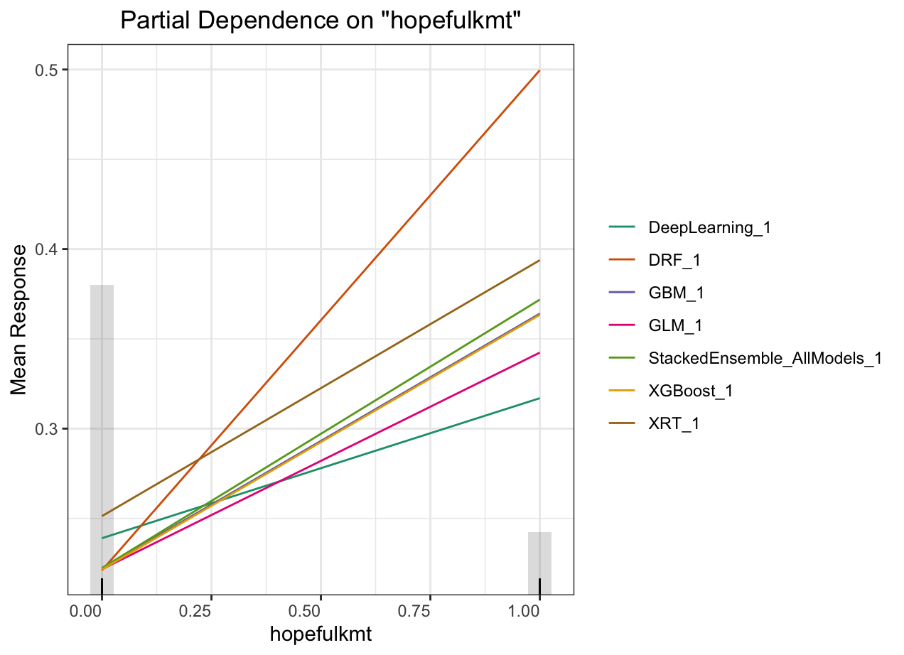
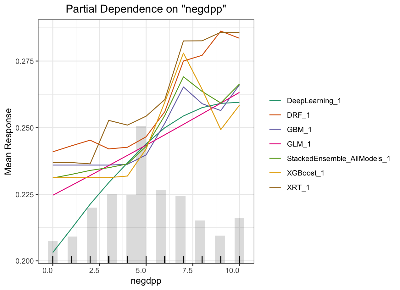
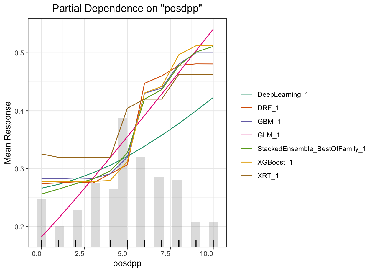
Partial dependence plot (PDP) gives a graphical depiction of the marginal effect of a variable on the response. The effect of a variable is measured in change in the mean response. PDP assumes independence between the feature for which is the PDP computed and the rest.
Automated Machine Learning: KMT
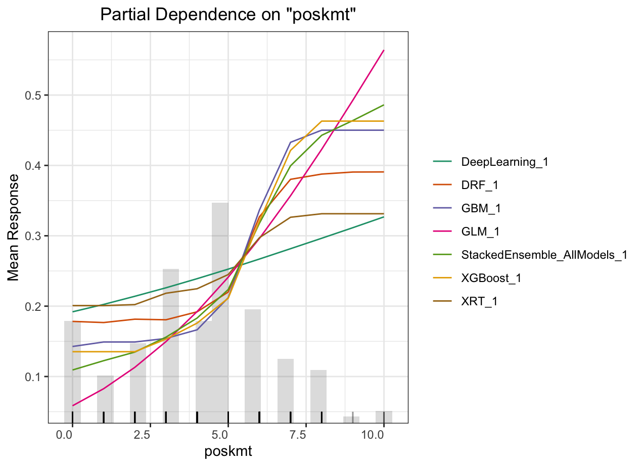
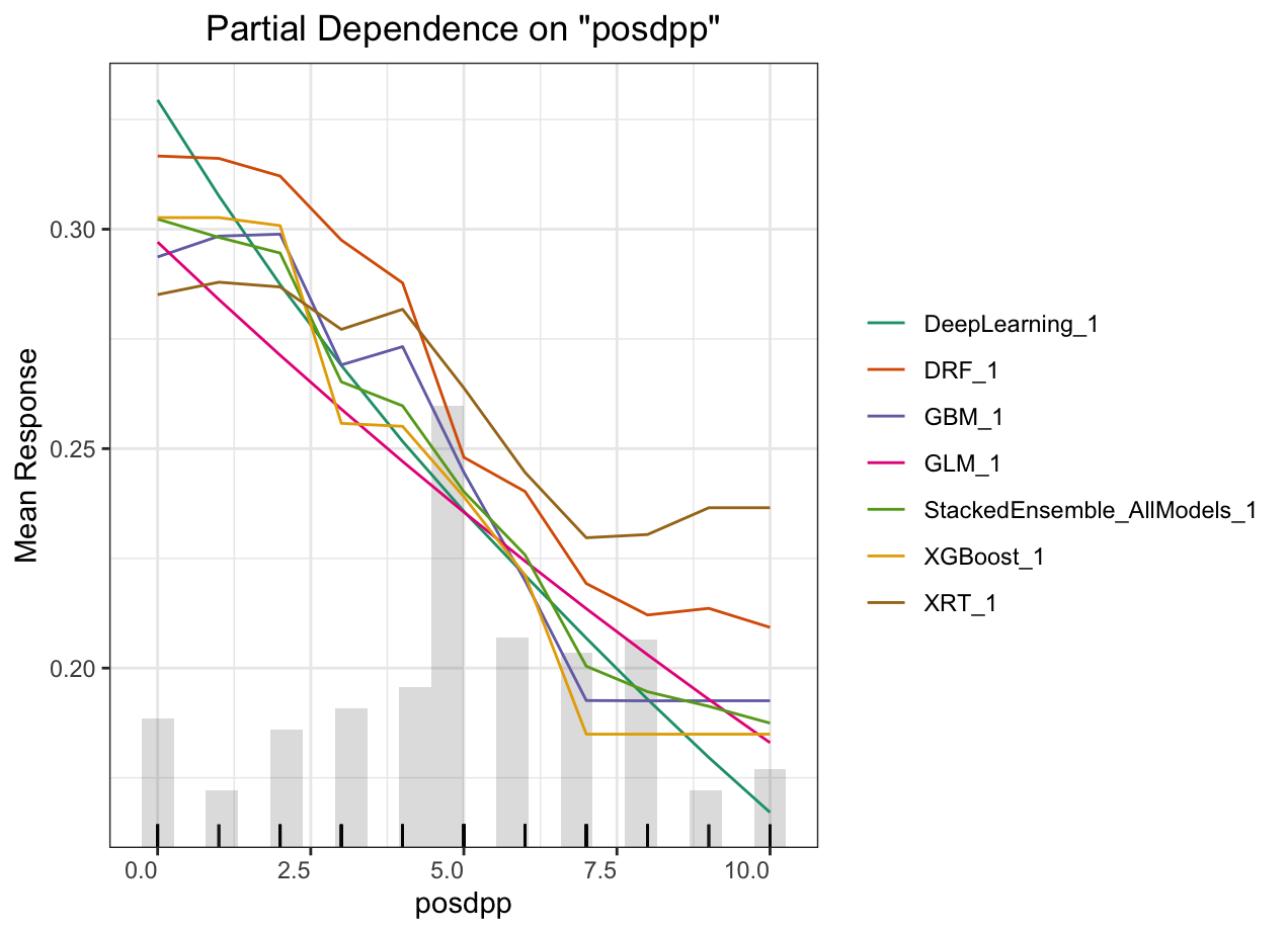
Automated Machine Learning: DPP
Automated Machine Learning: DPP
Automated Machine Learning: DPP