Gentle Introduction to Machine Learning
Karl Ho
School of Economic, Political and Policy Sciences
University of Texas at Dallas
Workshop prepared for International Society for Data Science and Analytics (ISDSA) Annual Meeting, Notre Dame University, June 2nd, 2022.
Supervised Learning
Overview
-
Supervised Learning
-
Regression
-
Classification
-
Tree-based Models
-
Overview
-
Linear Regression
-
Assessment of regression models
-
Multiple Linear Regression
-
Four important questions
-
Selection methods
-
Qualitative variables
-
Interaction terms
-
Nonlinear effects
-
Linear regression is a simple approach to supervised learning based on the assumption that the dependence of \(Y\) on \(X_{i}\) is linear.
True regression functions are never linear!
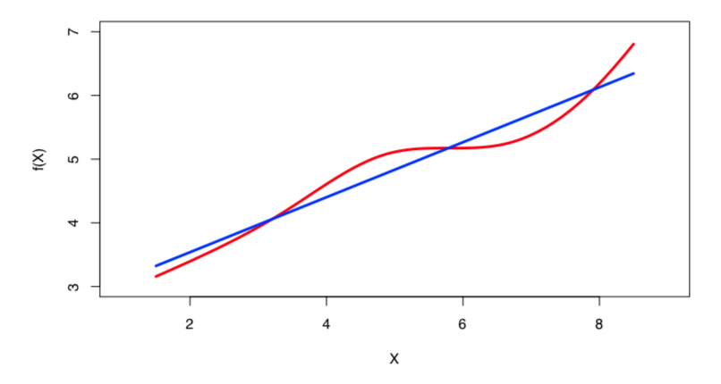
Real data are almost never linear due to different types of errors:
-
measurement
-
sampling
-
multiple covariates
Despite its simplicity, linear regression is very powerful and useful both conceptually and practically.
If prediction is the goal, how we can develop a synergy out of these data?
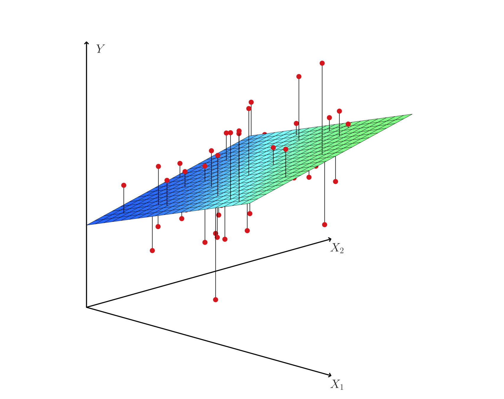
Hyperplane: multiple (linear) regression
Given some estimates \(\hat{\beta_{0}}\) and \(\hat{\beta_{1}}\) for the model coefficients, we predict dependent variable using:
\(Y\) = \(\beta_{0}\) + \(\beta_{1}\)\(X\) + \(\epsilon\)
where \(\beta_{0}\) and \(\beta_{1}\) are two unknown constants that represent the intercept and slope, also known as coefficients or parameters, and \(\epsilon\) is the error term.
\(\hat{y}\) = \(\hat{\beta_{0}}\) + \(\hat{\beta_{1}}\)\(x\)
Assume a model:
Given some estimates \(\hat{\beta_{0}}\) and \(\hat{\beta_{1}}\) for the model coefficients, we predict the dependent variable using:
where \(\hat{y}\) indicates a prediction of Y on the basis of X = x. The hat symbol denotes an estimated value.
\(\hat{y}\) = \(\hat{\beta_{0}}\) + \(\hat{\beta_{1}}\)\(x\)
\(\hat{y}\) = \(\hat{\beta_{0}}\) + \(\hat{\beta_{1}}\)\(x\)
Where is the \(e\)?
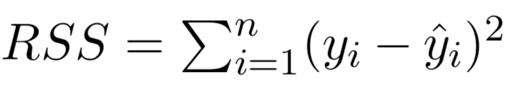
The least squares approach chooses \(\hat{\beta_{0}}\) and \(\hat{\beta_{1}}\) to minimize the RSS.
• Let \(\hat{y}_{i}\) = \(\hat{\beta_{0}}\) + \(\hat{\beta_{1}}\)\(x_{i}\) be the prediction for Y based on the \(i^{th}\) value of X. Then \(e_{i}\)=\(y_{i}\)-\(\hat{y}_{i}\) represents the \(i^{th}\) residual
• We define the residual sum of squares (RSS) as:
Estimation of the parameters by least squares
\(RSS\) = \(e_{1}^{2}\) + \(e_{2}^{2}\) + · · · + \(e_{n}^{2}\),
where and
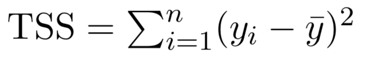
are the sample means.
The least squares approach chooses βˆ0 and βˆ1 to minimize the RSS. The minimizing values can be shown to be:
Estimation of the parameters by least squares

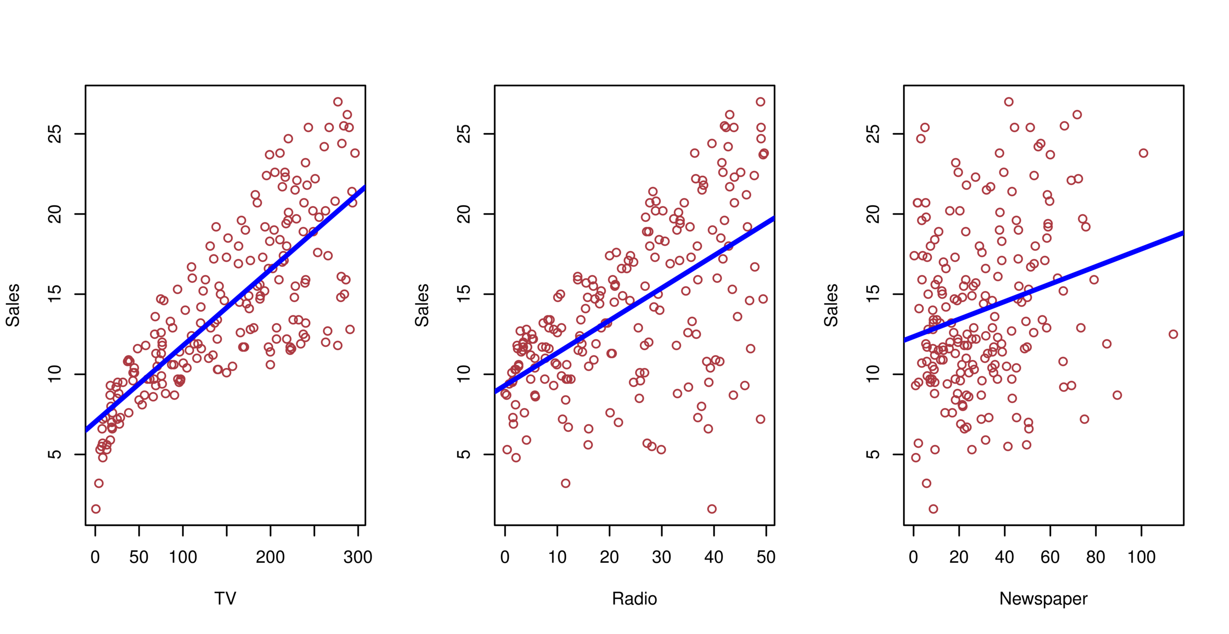
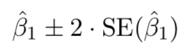
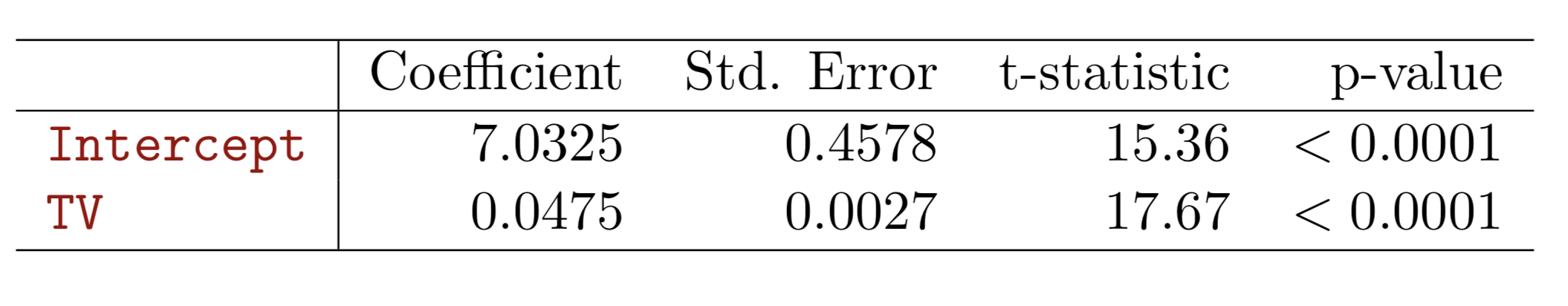
Advertising example
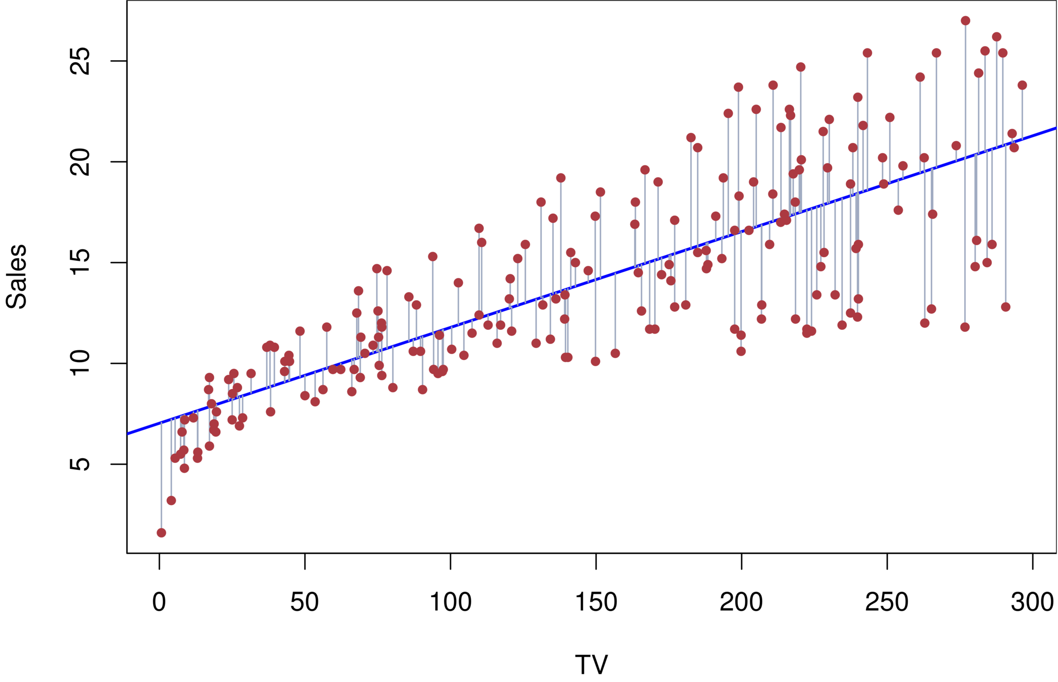
The least squares fit for the regression of sales onto TV. In this case a linear fit captures the essence of the relationship.
Assessment of regression model
-
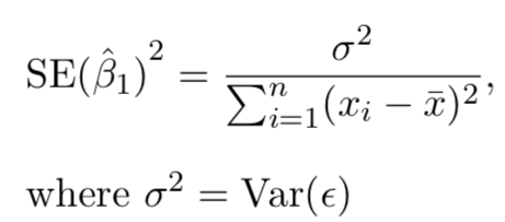
Standard errors
-
Using \(se\) and estimated coefficients, statistics such as t can be calculated for statistical significance:
-
\(t\)=\(\beta\)/\(se\)
-
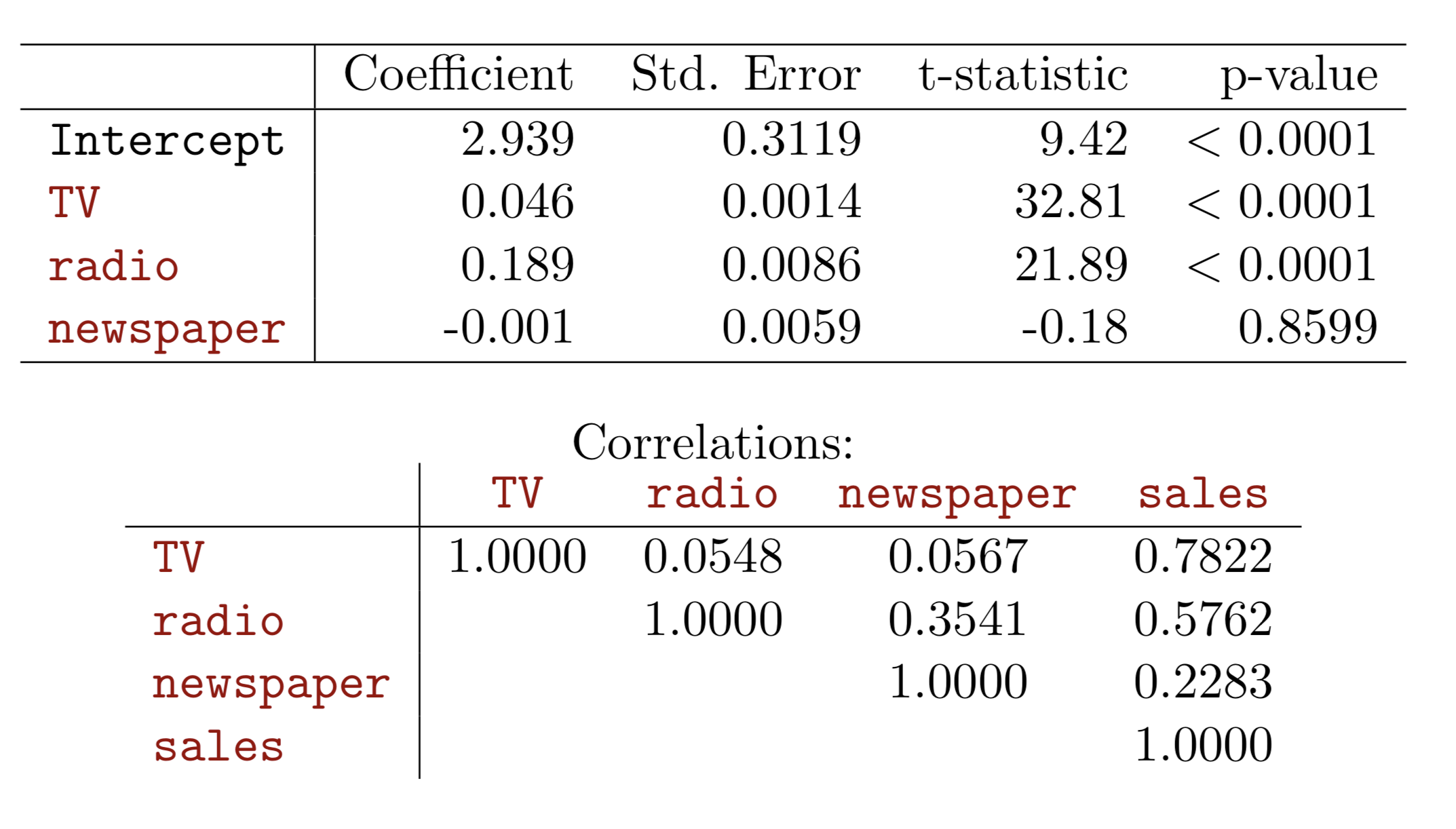
Multiple Linear regression
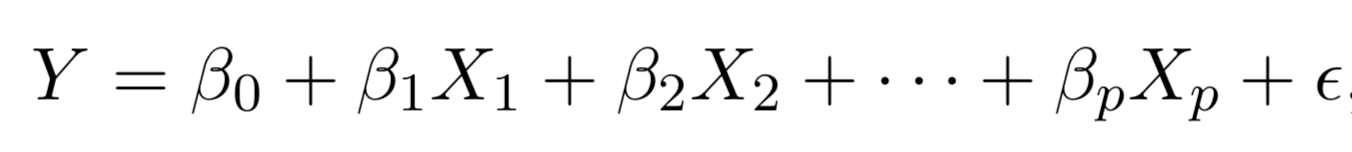
Multiple regression extends the model to multiple \(X\)'s or \(X_{p}\) where \(p\) is the number of predictors.
We interpret \(\beta_{j}\) as the average effect on Y of a one unit increase in \(X_{j}\), holding all other predictors fixed. In the advertising example, the model becomes:

Assessment of regression model
Standard errors can be used to compute confidence intervals. A 95% confidence interval is defined as a range of values such that with 95% probability, the range will contain the true unknown value of the parameter. It has the form:
Confidence interval are important for both frequentists and Bayesians to determine a predictor is "significant" or important in predicting y
Assessment of regression model
Assessment of regression model
Assessment of regression model
Model fit:
-
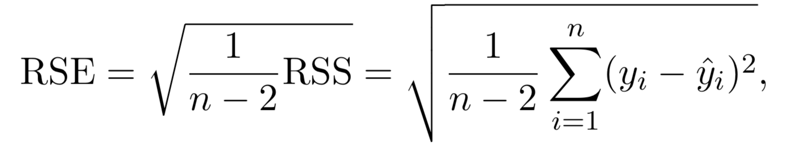
Residual Standard Error (RSS)
-
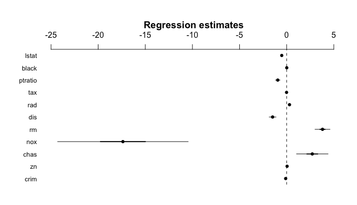
Each coefficient is estimated and tested separately, provided that there is no correlations among \(X\)'s
-
Interpretations such as “a unit change in \(X_{j}\) is associated with a \(\beta_{j}\) change in \(Y\) , while all the other variables stay fixed”, are possible.
-
Correlations amongst predictors cause problems:
-
The variance of all coefficients tends to increase, sometimes dramatically
-
Interpretations become hazardous — when \(X_{j}\)changes, everything else changes.
-
Multiple Linear regression
-
Problem of Multicollinearity
-
Claims of causality should be avoided for observational data.
Multiple Linear regression
Hyperplane: multiple (linear) regression
Multiple (linear) regression
Advertising example
-
Is at least one of the predictors \(X_1 , X_2 , . . . , X_p\) useful in predicting the response?
-
Do all the predictors help to explain Y, or is only a subset of the predictors useful?
-
How well does the model fit the data?
-
Given a set of predictor values, what response value should we predict, and how accurate is our prediction?
Four important questions
-
F-statistic to determine if at least one of the predictor's coefficient \(\beta_i\) is zero.
-
When there is a very large number of variables \((p > n)\), F-statistic cannot be used.
-
Can consider variable selection methods.
1. Is there a relationship between the response and predictors?
-
There are a total of \(2^p\) models that contain subsets of \(p\) variables.
- For example, when \(p=2\), there will be \(2^2=4\) models.
- model(1) with no variables
- model(2) with \(X_1\) only
- model(3) with \(X_2\) only
- model(4) with both \(X_1\) and \(X_2\).
- For example, when \(p=2\), there will be \(2^2=4\) models.
- When \(p\) becomes large, we need to consider variable selection methods:
- Forward selection: start with null model and add variable with lowest RSS then forward
- Backward selection: start with full model then remove variable with biggest p-value
- Mixed selection: start with null first forward then backward
2. Deciding on Important Variables
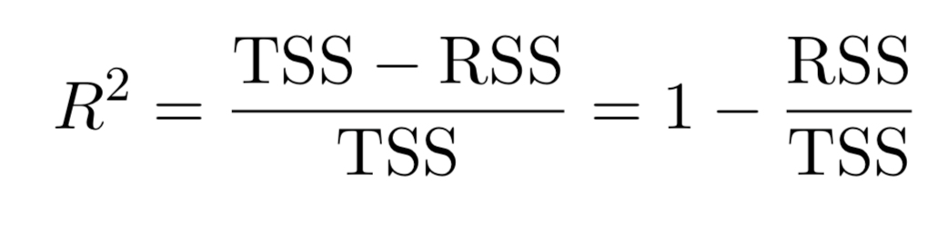
- Residual Standard Error (RSE) and \(R^2\), the fraction of variance explained can be used for model fit. The lower of RSE, the better. The higher the \(R^2\), the better.
- More predictors may not be always better. (e.g. Advertising example)
- Linear assumption is tested.
- Graphical analysis will help identifying more subtle relationship in different combination of RHS variables including interaction terms.
3. Model fit
3. Model fit

3. Model fit
- From the pattern of the residuals, we can see that there is a pronounced non-linear relationship in the data.
- The positive residuals (those visible above the surface), tend to lie along the 45-degree line, where TV and Radio budgets are split evenly.
- The negative residuals (most not visible), tend to lie away from this line, where budgets are more lopsided.
-
Three kinds of uncertainties
-
Reducible error: inaccurate coefficient estimates
-
Confidence intervals can be used.
-
-
Model bias: linearity assumption tested
-
Irreducible error: random error \(\epsilon\) in the model
-
Prediction intervals
-
Prediction intervals are always wider than confidence intervals, because they incorporate both the error in the estimate for \(f(X)\) (the reducible error) and the uncertainty as to how much an individual point will differ from the population regression plane (the irreducible error).
-
-
4. Prediction
With current computation power, we can test all subsets or combinations of the predictors in the regression models.
It will be costly, since there are \(2^{p}\) of them; it could be hitting millions or billions of models!
New technology or packages have been developed to perform such replicative modeling.
A Stata package mrobust by Young & Kroeger (2013)
What are important?
-
Begin with the null model — a model that contains an intercept but no predictors.
-
Fit \(p\) simple linear regressions and add to the null model the variable that results in the lowest RSS.
-
Add to that model the variable that results in the lowest RSS amongst all two-variable models.
-
Continue until some stopping rule is satisfied, for example when all remaining variables have a p-value above some threshold.
Selection methods: Forward selection
-
Start with all variables in the model.
-
Remove the variable with the largest p-value, that is, the variable that is the least statistically significant.
-
The new (\(p\) − 1)-variable model is fit, and the variable with the largest p-value is removed.
-
Continue until a stopping rule is reached. For instance, we may stop when all remaining variables have a significant p-value defined by some significance threshold.
Selection methods: backward selection
-
Mallow’s \(C_{p}\)
-
Akaike information criterion (AIC)
-
Bayesian information criterion (BIC)
-
Cross-validation (CV).
New selection methods
-
Categorical variables
-
Dichotomy (1,0)
-
class (1,2,3)
-
Leave one category as base category for comparison:
-
e.g. race, party
-
-
Qualitative variables
-
Treatment of two highly correlated variables
-
Multiplicative term--> Interaction term
-
Useful for multicollinearity problem
-
Hard to interpret and could lead to other problems
-
Hierarchy principle:
If we include an interaction in a model, we should also include the main effects, even if the p-values associated with their coefficients are not significant.
Interaction term/variables
Nonlinear effects
Nonlinear effects

-
Linear regression is a good starting point for predictive analytics
-
Simple
-
Highly interpretable
-
Error management
-
-
Limitations:
-
Numeric, quantitative variables
-
Need clear interpretations
-
other problems of regression?
-
-
Next: Classification and tree-based methods
Summary
Resampling involves repeatedly drawing samples from a training set and refitting a model of interest on each sample in order to obtain additional information about the fitted model.
Resampling
Such an approach allows us to obtain information that would not be available from fitting the model only once using the original training sample.
These methods refit a model of interest to samples formed from the training set, in order to obtain additional information about the fitted model.
Resampling
Resampling provide estimates of test-set prediction error, and the standard deviation and bias of our parameter estimates
Test error is the average error that results from using a statistical learning method to predict the response on new observations that were not used in training the method.
Test error
Training error is the error calculated by applying the statistical learning method to the observations used in its training.
Training error
The training error rate is often quite different from the test error rate, and the former can dramatically underestimate the latter.
Training- versus Test-Set Performance
Source: ISLR Figure 2.7, p. 25
Again, beware of the evil of overfitting!
Flexibility vs. Interpretability
Source: ISLR Figure 2.7, p. 25
In general, as the flexibility of a method increases, its interpretability decreases.
Cross-validation estimates the test error associated with a given statistical learning method to evaluate performance, or to select the appropriate level of flexibility.
Cross-validation (CV)
The process of evaluating a model’s performance is known as model assessment.
The process of selecting the proper level of flexibility for a model is called model selection.
-
Randomly divide the sample into two parts: a training set and a hold-out set (validation).
-
Fit on the model with the training set to predict the responses for the observations in the validation set.
-
The resulting validation-set error provides an estimate of the test error (using \(MSE\)).
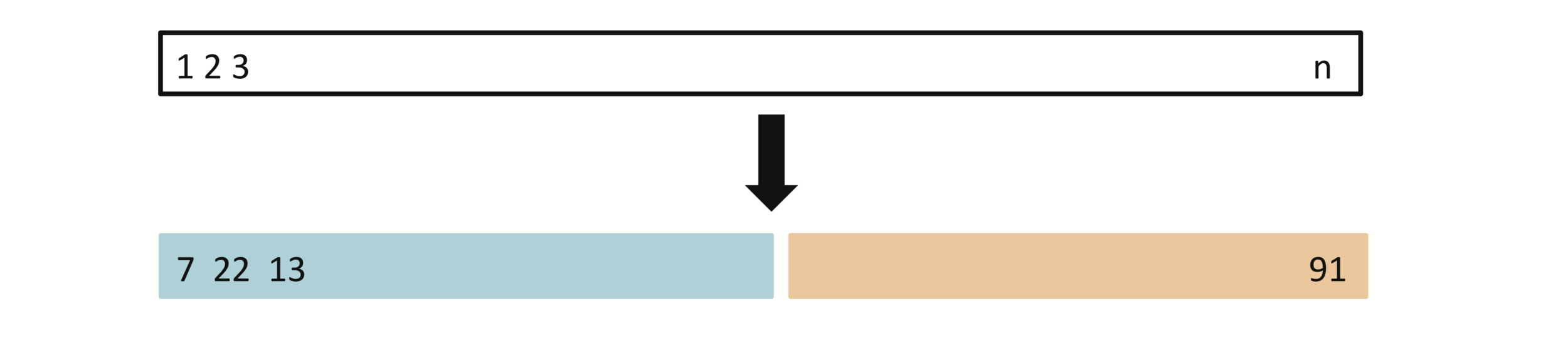
Validation-set approach
$$ MSE=\frac{1}{n} \sum_{i=1}^n(y_{i}-\hat{f}(x_{i}))^2 $$
Mean Squared Error (MSE)
Mean Squared Error is the extent to which the predicted response value for a given observation is close to
the true response value for that observation.
where \(\hat{f}(x_{i})\) is the prediction that \(\hat{f}\) gives for the \(i^{th}\) observation.
The MSE will be small if the predicted responses are very close to the true responses, and will be large if for some of the observations, the predicted and true responses differ substantially.
Validation-set approach
Random splitting into two halves: left part is training set, right part is validation set
Illustration: linear vs. polynomial
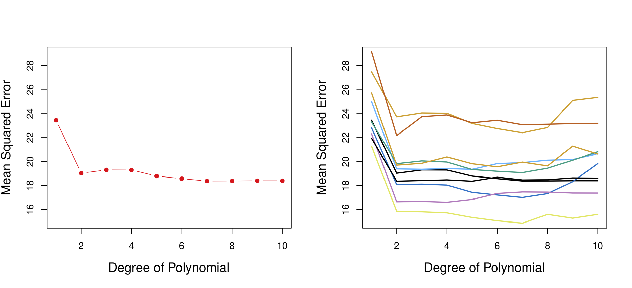
Linear vs. Quadratic vs. Cubic
Validation 10 times
Conclusion: Quadratic form is the best.
-
Validation estimate of test error rate can be highly variable, depending on included observations in the training set (extreme observations included??).
-
Only a subset of the observations are used to fit the model, the validation set error rate may tend to overestimate the test error rate for the model fit on the entire data set.
Validation-set approach drawbacks
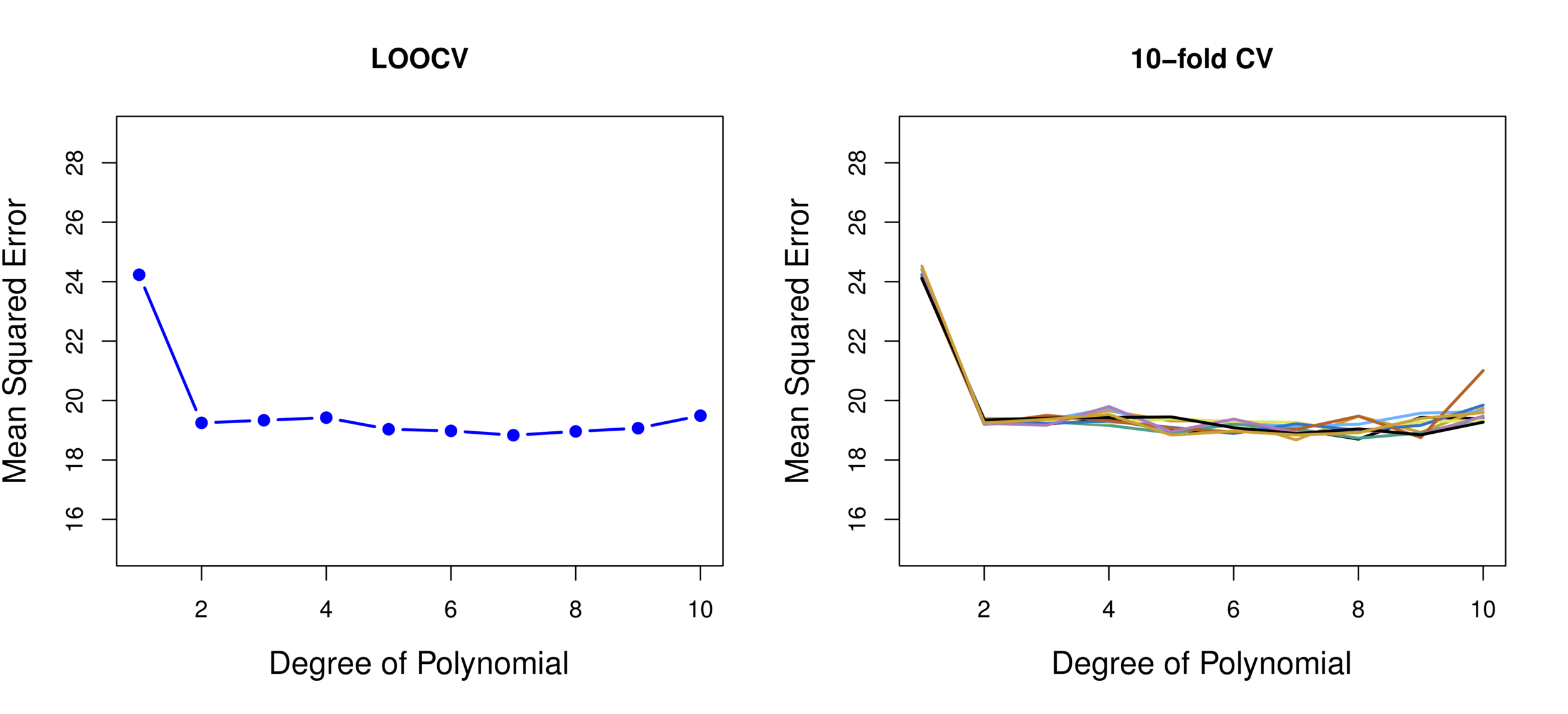
Leave-One-Out Cross-Validation
(LOOCV)
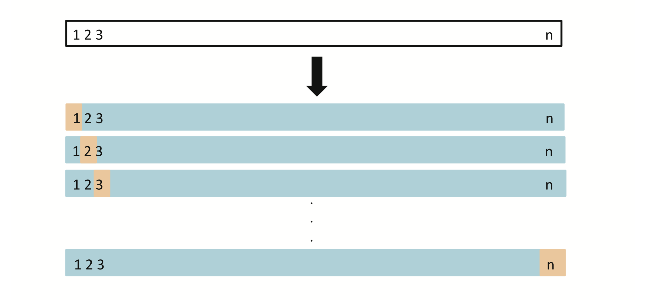
A set of \(n\) data points is repeatedly split into a training set containing all but one observation, and a validation set that contains only that observation. The test error is then estimated by averaging the \(n\) resulting \(MSE\)’s. The first training set contains all but observation 1, the second training set contains all but observation 2, and so forth.
K-fold Cross-validation
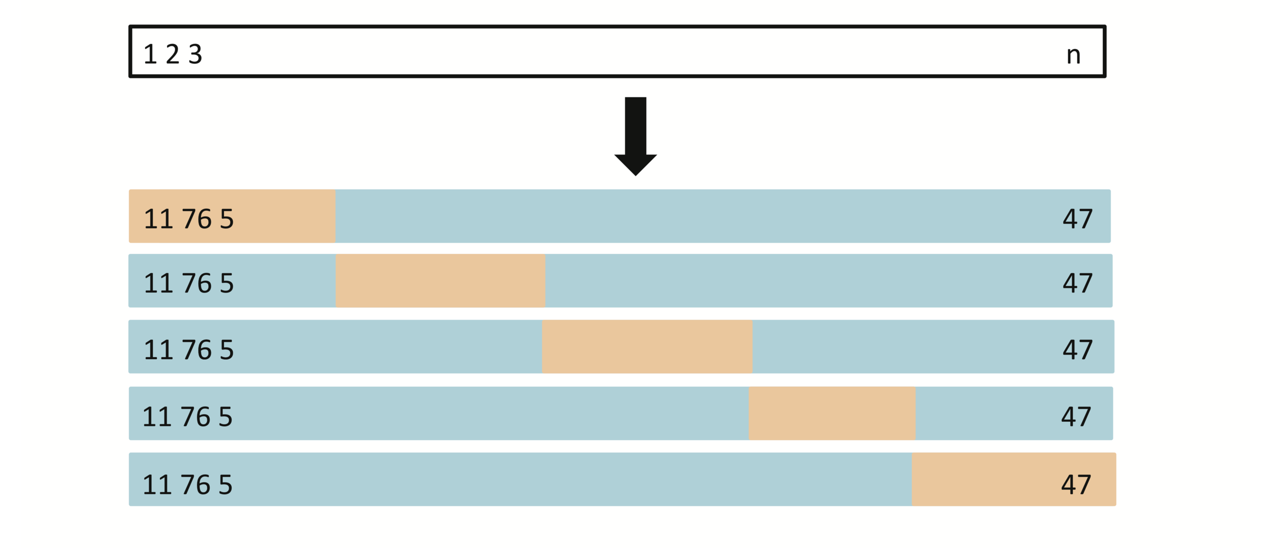
A set of \(n\) observations is randomly split into five non-overlapping groups. Each of these fifths acts as a validation set, and the remainder as a training set. The test error is estimated by averaging the five resulting \(MSE\) estimates.
K-fold Cross-validation
LOOCV sometimes useful, but typically doesn’t shake up the data enough. The estimates from each fold are highly correlated and hence their average can have high variance.
Consider a simple classifier applied to some two-class data:
-
Starting with 5000 predictors and 50 samples, find the 100 predictors having the largest correlation with the class labels.
-
We then apply a classifier such as logistic regression, using only these 100 predictors.
Proper way of cross-validation
-
Can we apply cross-validation in step 2, forgetting about step 1?
-
This would ignore the fact that in Step 1, the procedure has already seen the labels of the training data, and made use of them. This is a form of training and must be included in the validation process.
-
It is easy to simulate realistic data with the class labels independent of the outcome, so that true test error =50%, but the CV error estimate that ignores Step 1 is zero!
Proper way of cross-validation
-
Repeatedly sampling observations from the original data set.
-
Randomly select \(n\) observations with replacement from the data set.
-
In other words, the same observation can occur more than once in the bootstrap data set.
Bootstrap
The use of the term \(bootstrap\) derives from the phrase to pull oneself up by one’s bootstraps (improve one's position by one's own efforts), widely thought to be based on one of the 18th century “The Surprising Adventures of Baron Munchausen” by Rudolph Erich Raspe:
Bootstrap
The Baron had fallen to the bottom of a deep lake. Just when it looked like all was lost, he thought to pick himself up by his own bootstraps.
Bootstrap
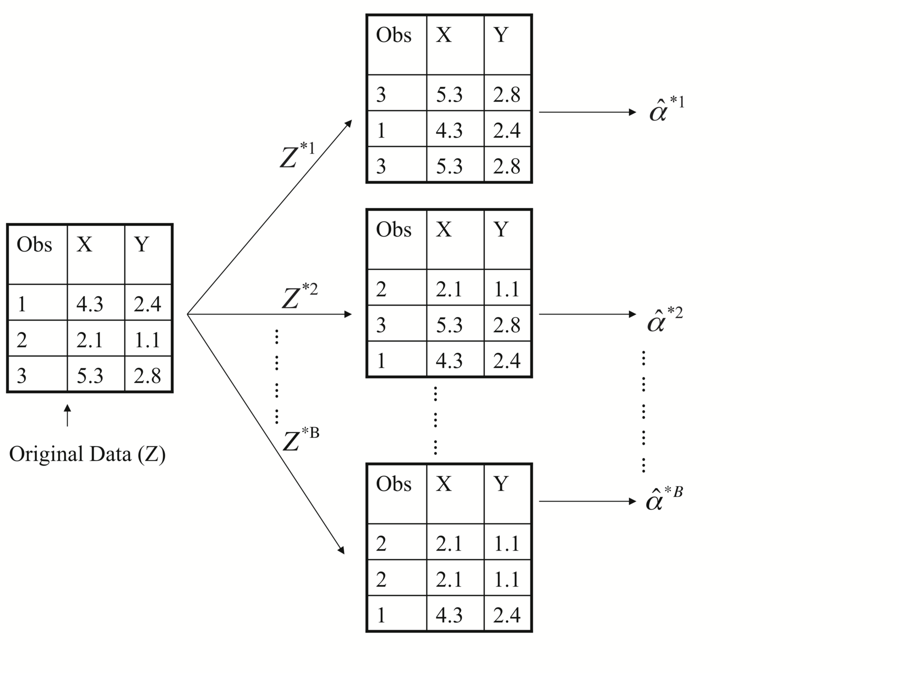
Each bootstrap data set contains \(n\) observations, sampled with replacement from the original data set. Each bootstrap data set is used to obtain an estimate of \(\alpha\)
Bootstrap
Bootstrap vs. Jackknife
Bootstrap: replacement resampling
Jackknife (John Tukey) is a resampling technique especially useful for variance and bias estimation
Jackknife: resampling by leaving out observation
[1,2,3,4,5], [2,5,4,4,1], [1,3,2,5,5],......
[1,2,3,4,5], [2,5,4,1], [1,2,5],......
-
Suppose that we invest a fixed sum of money in two financial assets that yield returns of \(X\) and \(Y\) , respectively, where \(X\) and \(Y\) are random quantities (Portfolio dataset).
-
A fraction \(\alpha\) of the money invested in \(X\), and the remaining \(1-\alpha\) will be in \(Y\)
-
Naturally, we want to choose an \(\alpha\) that minimizes the total risk, or variance, of our investment. In other words, we want to minimize \(Var(\alpha X + (1 − \alpha) Y)\).
Illustration: Portfolio example
-
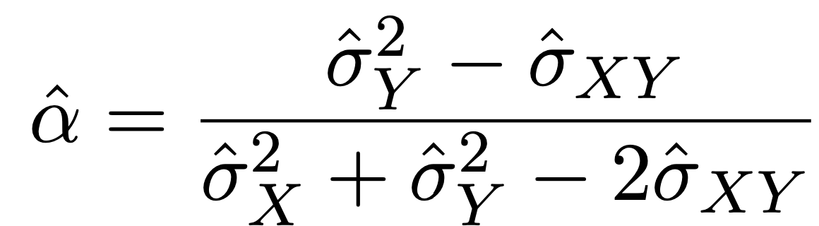
One can show that the value that minimizes the risk is given by
Illustration: Portfolio example

-
But the values of \(\sigma_{x}^2\), \(\sigma_{y}^2\) , and \(\sigma_{xy}\) are unknown.
-
We can compute estimates for these quantities, \(\hat{\sigma}_{x}^2\) , \(\hat{\sigma}_{y}^2\) , and \(\hat{\sigma}_{xy}\) , using a data set that contains measurements for X and Y.
-
We can then estimate the value of \(\alpha\) that minimizes the variance of our investment using:
Illustration: Portfolio example
-
To estimate the standard deviation of \(\hat{\alpha}\), we repeated the process of simulating 100 paired observations of X and Y , and estimating \(\alpha\) 1,000 times.
-
We thereby obtained 1,000 estimates for \(\alpha\), which we can call \(\hat{\alpha}_{1}\) ,\(\hat{\alpha}_{2}\) ,...,\(\hat{\alpha}_{1000}\).
-
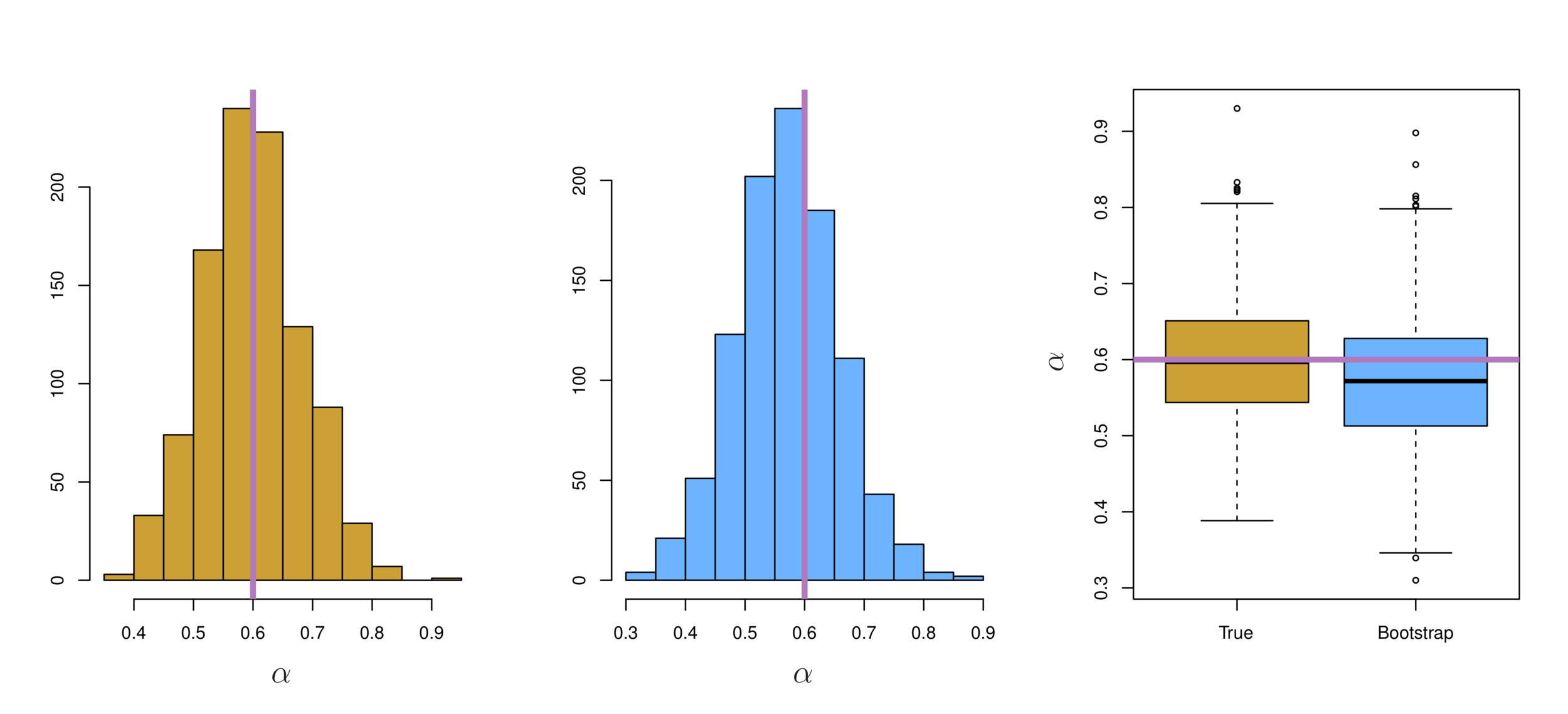
For these simulations the parameters were set to \(\sigma_{x}^2\) = 1,\(\sigma_{y}^2\) = 1.25, and \(\sigma_{xy}\) = 0.5, and so we know that the true value of \(\alpha\) is 0.6.
Illustration: Portfolio example
-
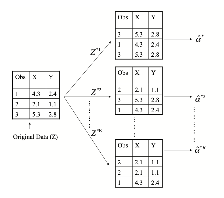
Denoting the first bootstrap data set by \(Z^{∗1}\), we use \(Z^{∗1}\) to produce a new bootstrap estimate for \(\alpha\), which we call \(\hat{\alpha}^{∗1}\)
-
This procedure is repeated \(B\) times for some large value of \(B\)(say 100 or 1,000 times), in order to produce \(B\) different bootstrap data sets, \(Z^{∗1}\),\(Z^{∗2}\),...,\(Z^{∗B}\), and \(B\) corresponding \(\alpha\) estimates, \(\hat{\alpha}^{∗1}\), \(\hat{\alpha}^{∗2}\),..., \(\hat{\alpha}^{∗B}\).
Illustration: Portfolio example
-
We estimate the standard error of these bootstrap estimates using the formula:\[SE_B(\hat{\alpha})=\sqrt{\frac{1}{B-1}\sum_{r=1}^{B}(\hat{\alpha}^{*r}-\bar{\hat{\alpha}^*})^2}\]
-
This serves as an estimate of the standard error of \(\hat{\alpha}\) estimated from the original data set. For this example \(SE_B(\hat{\alpha}) = 0.087\).
Illustration: Portfolio example
Left: Histogram of the estimates of \(\alpha\) obtained by generating 1,000 simulated data sets from the true population. Center: A histogram of the estimates of \(\alpha\)obtained from 1,000 bootstrap samples from a single data set. Right: Boxplots of estimates of \(\alpha\) displayed in the left and center panels. In each panel, the pink line indicates the true value of \(\alpha\).
Illustration: Portfolio example
-
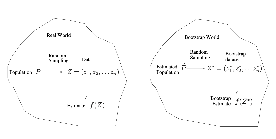
we cannot generate new samples from the original population.
-
However, the bootstrap approach allows us to use a computer to mimic the process of obtaining new data sets, so that we can estimate the variability of our estimate without generating additional samples.
In reality....
-
In more complex data situations, figuring out the appropriate way to generate bootstrap samples can require some thought.
-
For example, if the data is a time series, we can’t simply sample the observations with replacement (why not?).
-
We can instead create blocks of consecutive observations, and sample those with replacements. Then we paste together sampled blocks to obtain a bootstrap dataset.
The bootstrap in general
-
Primarily used to obtain standard errors of an estimate.
-
Also provides approximate confidence intervals for a population parameter. For example, looking at the histogram in the previous illustration, the 5% and 95% quantiles of the 1000 values is (.43, .72) which represents an approximate 90% confidence interval for the true \(\alpha\).
-
This interval is called a Bootstrap Percentile confidence interval. It is the simplest method (among many approaches) for obtaining a confidence interval from the bootstrap.
Other uses of the bootstrap
Classification:
- Dealing with qualitative variables such as groups or categories or survival or not.
- Recognition methods, AI
Overview
Qualitative variables take values in an unordered set C, such as:
-
\(Party ID \in {Democrats, Republican, Independent}\)
-
\(Voted \in {Yes, No}\).
Classification
Given a feature vector \(X\) and a qualitative response \(Y\) taking values in the set \(C\), the classification task is to build a function \(C(X)\) that takes as input the feature vector \(X\) and predicts its value for \(Y\) ; i.e. \(C(X) \in C\).
-
From prediction point of view, we are more interested in estimating the probabilities that \(X\) belongs to each category in \(C\).
-
For example, voter \(X\) will vote for a Republican candidate or will a student credit card owner default.
-
We cannot exactly say this voter will 100% vote for this party, yet we can say by so much chance she will do so.
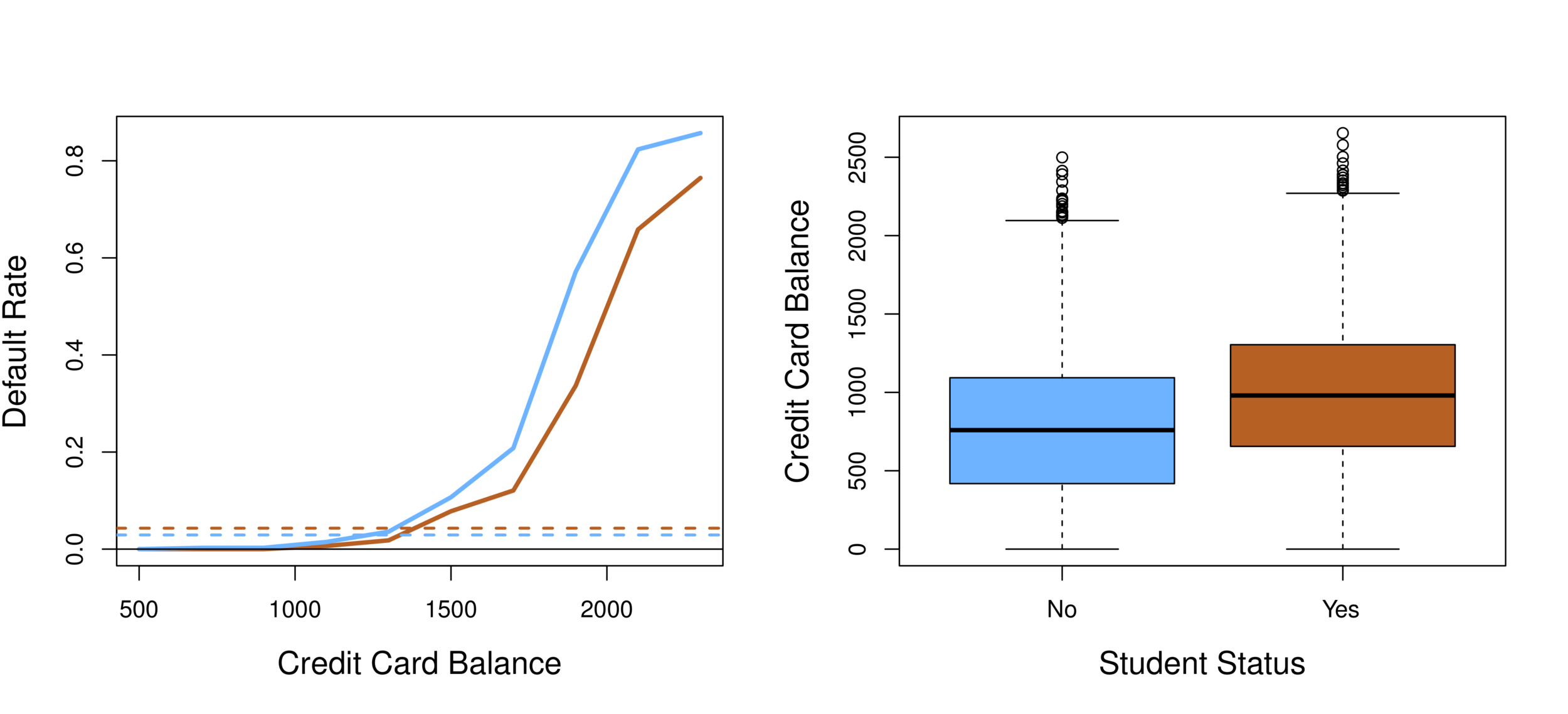
Classification
-
Orange: default, Blue: not
-
Overall default rate: 3%
-
Higher balance tend to default
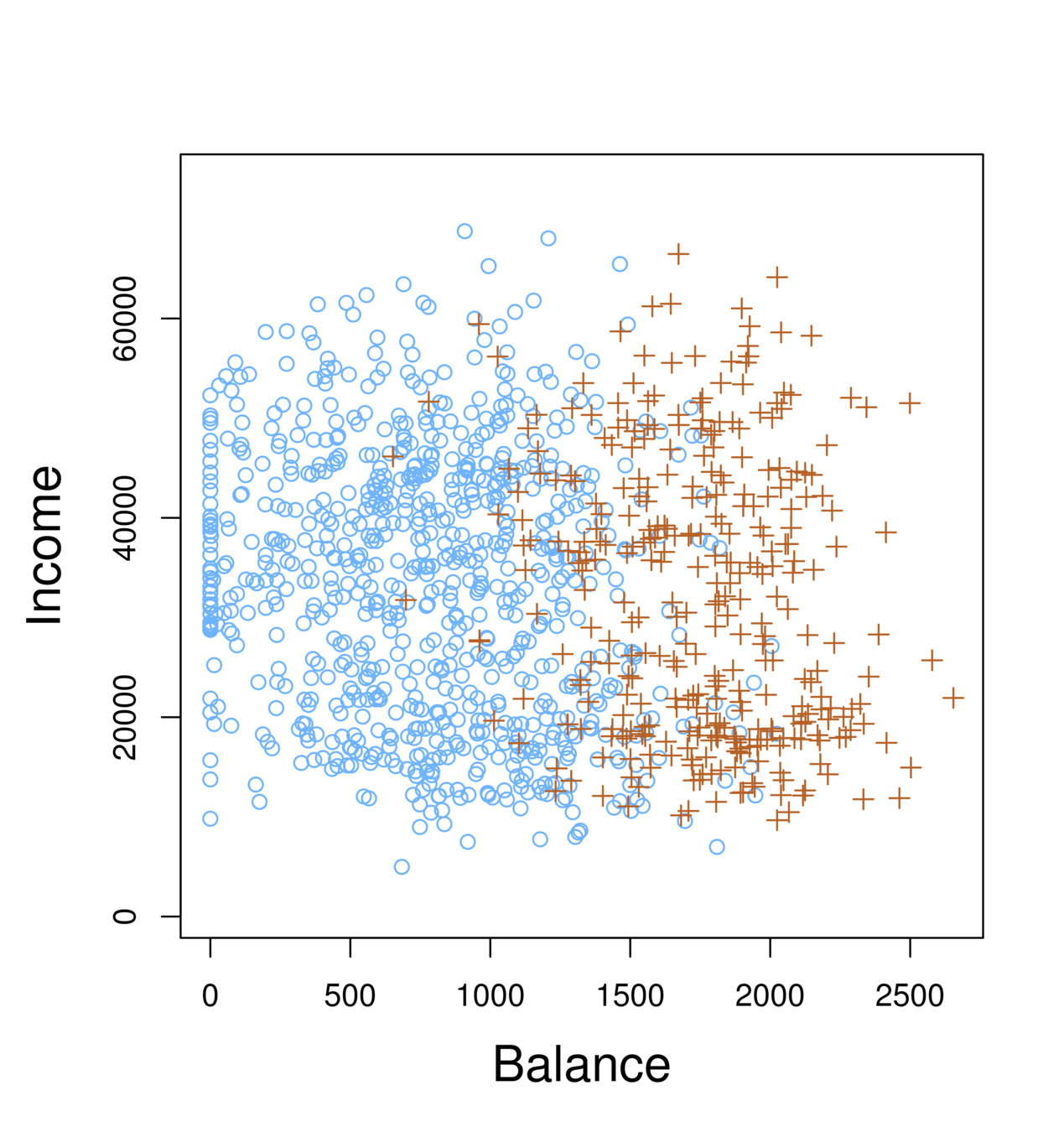
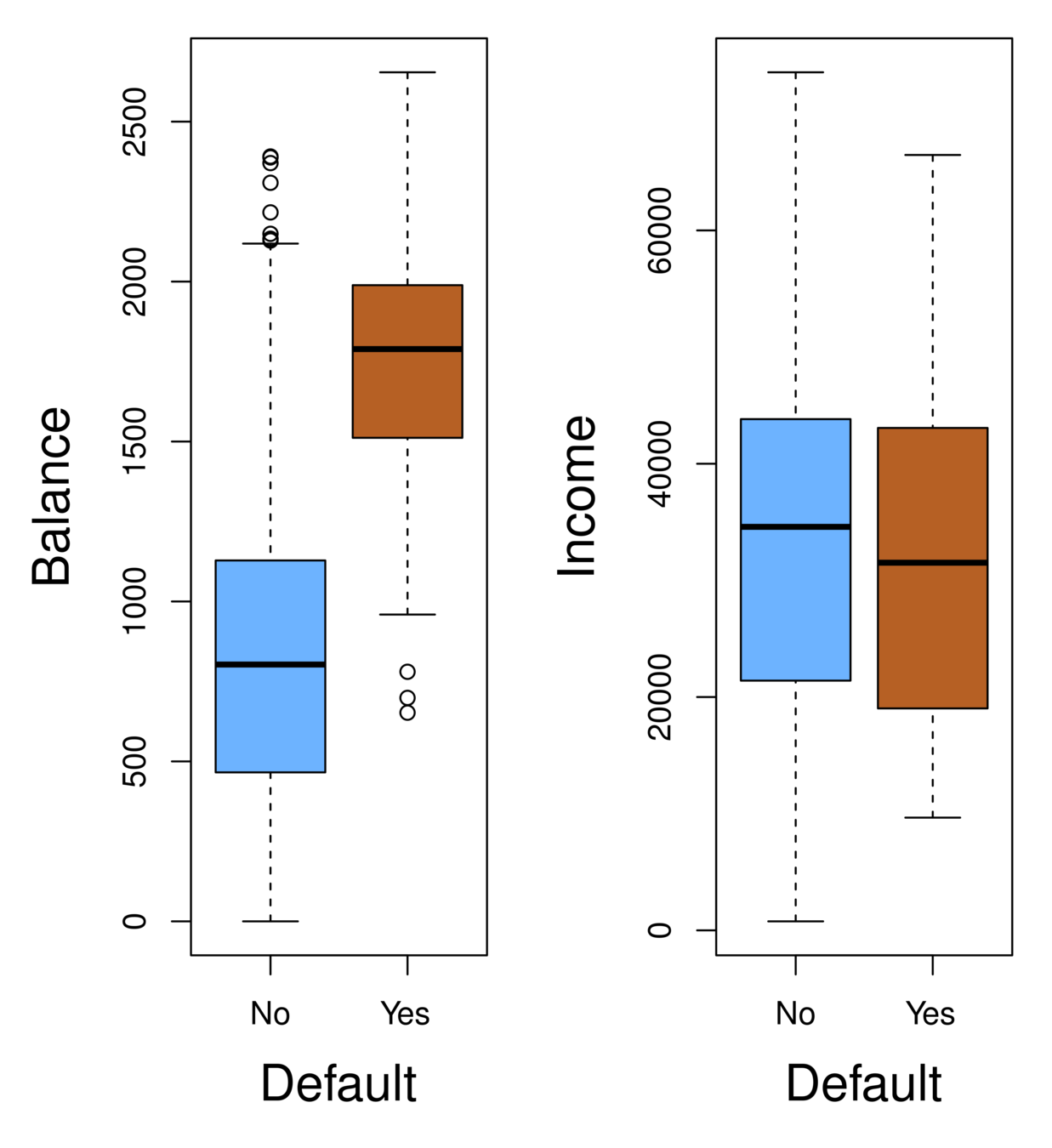
-
Income has any impact?
-
Mission:
-
Predict default \((Y )\) using balance \(X_1\) and income \(X_2\).
-
Since \(Y\) is not quantitative, the simple linear regression model is not appropriate.
-
Consider \(Y\) being three categories, linear regression cannot be used given the lack of order among these categories.
-
Classification
-
Can linear regression be used on two category variable (e.g. 0,1)?
-
For example, voted (1) or not voted(0), cancer (1) or no cancer (0)
-
Regression can still generate meaningful results.
-
Question: What does zero (0) mean? How to assign 0 and 1 to the categories?
-
For example, Republican and Democrat, pro-choice and pro-life
Classification
-
Instead of modeling the numeric value of Y responses directly, logistic regression models the probability that Y belongs to a particular category.
Logistic Regression
-
Linear regression vs. Logistic regression
-
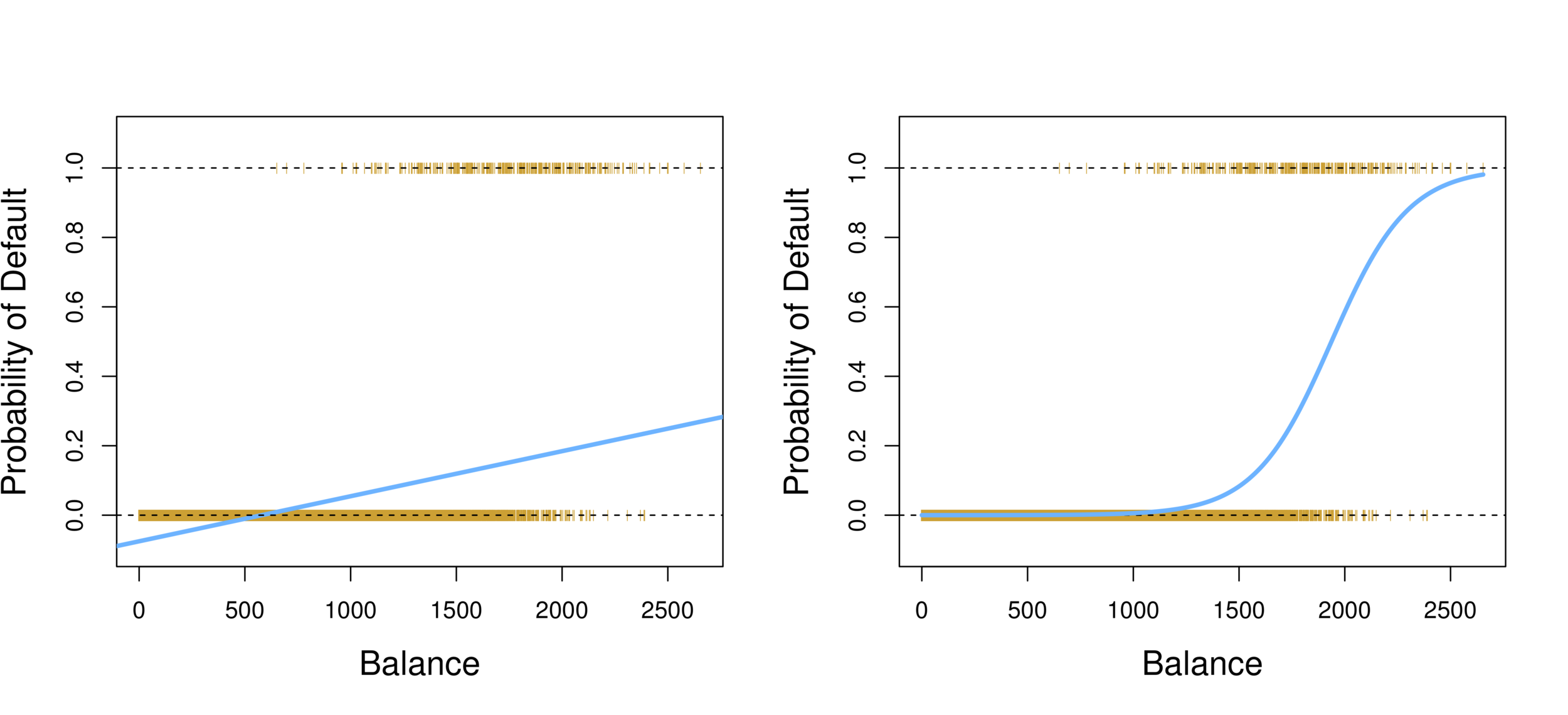
Using linear regression, predictions can go out of bound!
Logistic Regression
-
Probability of default given balance can be written as:
\(Pr(default = Yes | balance)\).
-
Prediction using \(p(x)>.5\), where x is the predictor variable (e.g. balance)
-
Can set other or lower threshold (e.g. \(p(x)>.3\))
Logistic Regression
-
To model \(p(X)\), we need a function that gives outputs between 0 and 1 for all values of \(X\).
-
In logistic regression, we use the logistic function,
Logistic Model
-
The numerator is called the odds
-
Which is the same as:
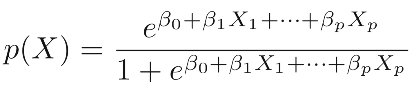
\[p(X) = \frac{e ^ {\beta_0+\beta_1X}}{1+e ^ {\beta_0+\beta_1X}}\]
\[e^{\beta_0+\beta_1X}\]
\[\frac{p(X)}{1-p(X)}\]
-
\(e ≈ 2.71828\) is a mathematical constant [Euler’s number.] No matter what values \(\beta_0\), \(\beta_1\) or \(X\) take, \(p(X)\) will have values between 0 and 1.
-
The odds can be understood as the ratio of probabilities between on and off cases (1,0)
-
For example, on average 1 in 5 people with an odds of 1/4 will default, since \(p(X) = 0.2\) implies an odds of
\(0.2/(1-0.2) = 1/4\).
Logistic Model
\[\frac{p(X)}{1-p(X)}\]
-
Taking the log of both sides, we have:
Logistic Model
-
The left-hand side is called the log-odds or logit, which can be estimated as a linear regression with X.
-
Note that however, \(p(X)\) and \(X\) are not in linear relationship.
\[\frac{p(X)}{1-p(X)}=e^{\beta_0+\beta_1X}\]
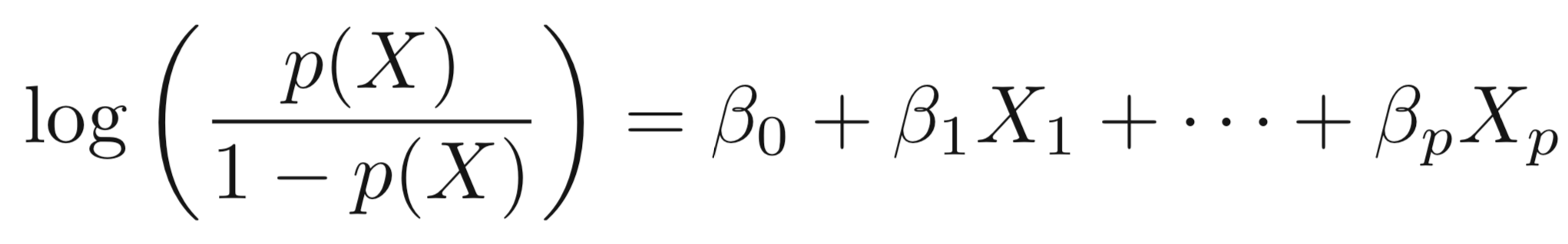
\[log(\frac{p(X)}{1-p(X)})=\beta_0+\beta_1X\]
-
Logistic Regression can be estimated using Maximum Likelihood.
-
We seek estimates for \(\beta_{0}\) and \(\beta_{1}\) such that the predicted probability \(\hat{p}(x_{i})\) of default for each individual, using \(p(X) = \frac{e ^ {\beta_0+\beta_1X}}{1+e ^ {\beta_0+\beta_1X}}\) corresponds as closely as possible to the individual’s observed default status.
-
In other words, we try to find \(\beta_{0}\) and \(\beta_{1}\)such that plugging these estimates into the model for \(p(X)\) yields a number close to one (1) for all individuals that fulfill the on condition (e.g. default) and a number close to zero (0) for all individuals of off condition (e.g. not default).
Logistic Regression
-
Maximum likelihood to estimate the parameters: \[\ell(\beta_0, \beta) = \prod_{i:y_i=1}p(x_i)\prod_{i:y_i=0}(1-p(x_i))\]
-
This likelihood gives the probability of the observed zeros and ones in the data. We pick \(\beta_0\) and \(\beta_1\) to maximize the likelihood of the observed data.
- Most statistical packages can fit linear logistic regression models by maximum likelihood. In R, we use the glm function.
Logistic Regression:
Maximum Likelihood
Logistic Regression
Coefficients:
              Estimate Std. Error z value Pr(>|z|)
(Intercept) -1.065e+01  3.612e-01  -29.49   <2e-16 ***
balance      5.499e-03  2.204e-04   24.95   <2e-16 ***
Output:
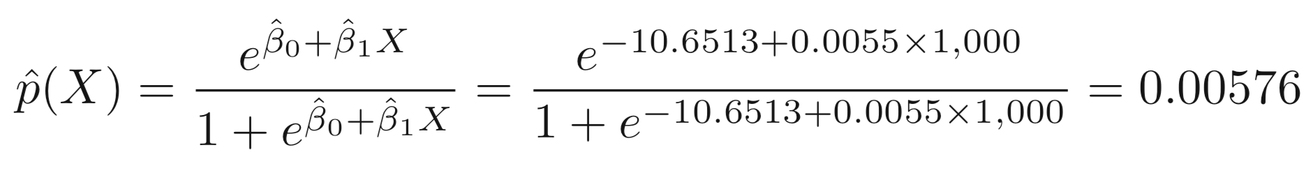
Suppose an individual has a balance of $1,000,
glm.fit=glm(default~balance,family=binomial)
summary(glm.fit)
Logistic Regression
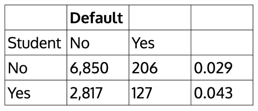
| Default | |||
|---|---|---|---|
| Student | No | Yes | |
| No | 6,850 | 206 | 0.029 |
| Yes | 2,817 | 127 | 0.043 |
How about the case of students?
> table(student,default)
       default
student   No  Yes
    No  6850  206
    Yes 2817  127
We can actually calculate by hand the rate of default among students:
Logistic Regression
Coefficients:
            Estimate Std. Error z value Pr(>|z|)
(Intercept) -3.50413    0.07071  -49.55  < 2e-16 ***
studentYes   0.40489    0.11502    3.52 0.000431 ***

glm.sfit=glm(default~student,family=binomial)
summary(glm.sfit)-
We can extend the Logistic Regression to multiple right hand side variables.
Multiple Logistic Regression
Multiple Logistic Regression
> glm.nfit=glm(default~balance+income+student,data=Default,family=binomial)
> summary(glm.nfit)
Coefficients:
              Estimate Std. Error z value Pr(>|z|)
(Intercept) -1.087e+01  4.923e-01 -22.080  < 2e-16 ***
balance      5.737e-03  2.319e-04  24.738  < 2e-16 ***
income       3.033e-06  8.203e-06   0.370  0.71152
student[Yes]  -6.468e-01  2.363e-01  -2.738  0.00619 **
Why student becomes negative? What does this mean?
Multiple Logistic Regression
Confounding effect: when other predictors in model, student effect is different.
- Students tend to have higher balances than non-students, so their marginal default rate is higher than for non-students.
- But for each level of balance, students default less than non-students.
- Multiple logistic regression can show this with other variables included (controlled for).
Discriminant Analysis
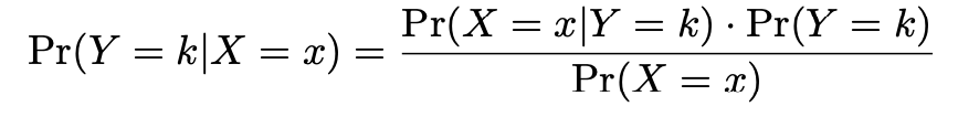
Logistic regression involves directly modeling \(Pr(Y = k|X = x)\) using the logistic function. In English, we say that we model the conditional distribution of the response Y, given the predictor(s) \(X\).
This is called the Bayes classifier.
In a two-class problem where there are only two possible response values, say class 1 or class 2, the Bayes classifier corresponds to predicting class 1 if \(Pr(Y = 1|X = x_0) > 0.5\) , and class 2 otherwise.
Discriminant Analysis
Suppose that we wish to classify an observation into one of \(K\) classes, where
\(K ≥ 2\).
Let \(\pi_{k}\) represent the overall or prior probability that a randomly chosen observation comes from the \(k^{th}\)class; this is the probability that a given observation is associated with the \(k^{th}\) category of the response variable \(Y\) .
Discriminant Analysis
By Bayes theorem:
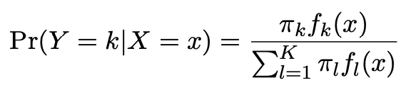
where \(\pi_{k}\) = \(Pr(Y = k)\) is the marginal or prior probability for class k,
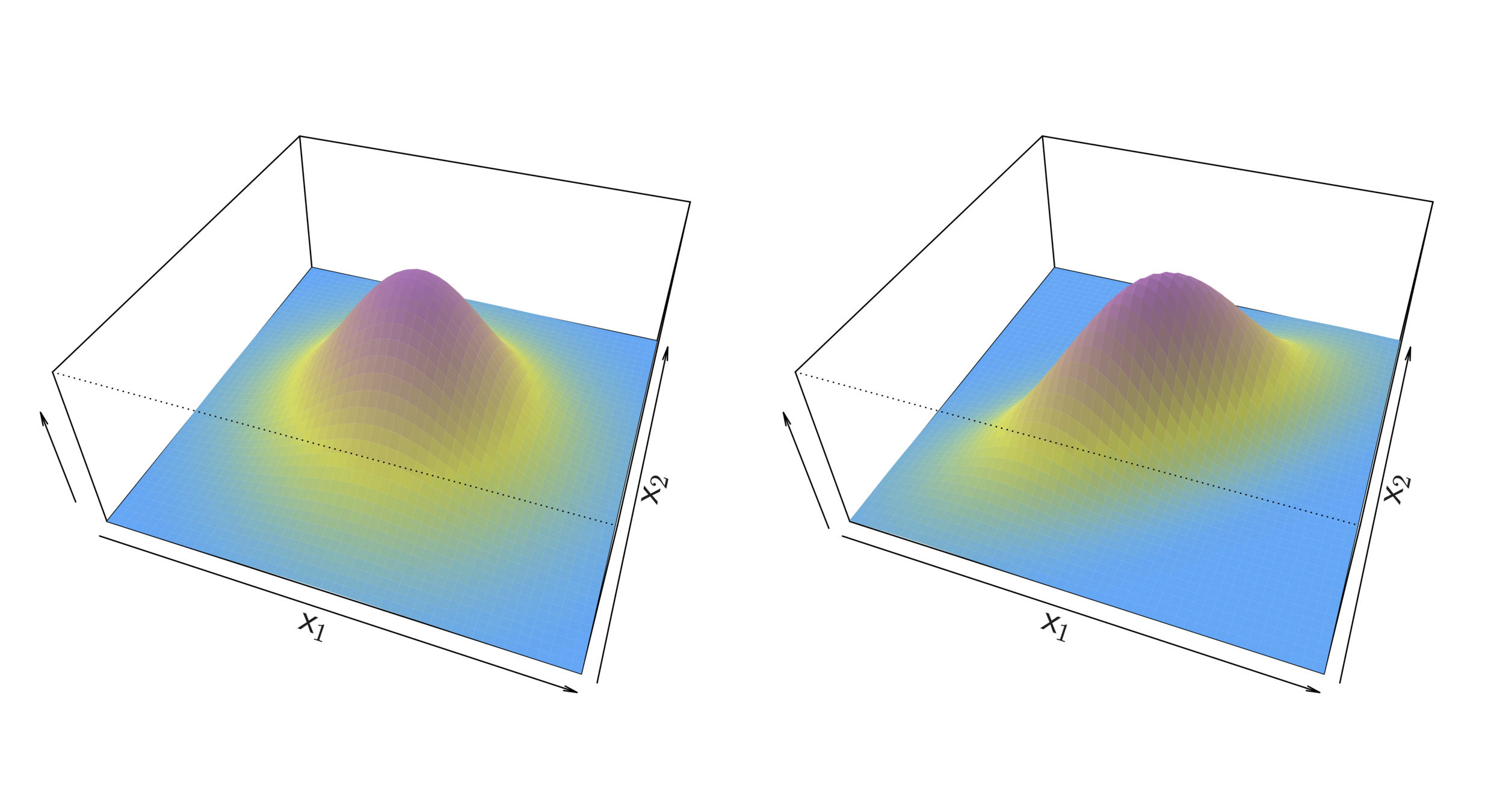
\(f_{k}(x)\)=\(Pr(X=x|Y=k)\) is the density for \(X\) in class \(k\). Here we will use normal densities for these, separately in each class.
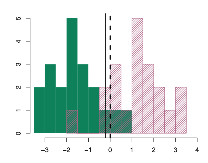
Discriminant Analysis
We classify a new point according to which density is highest.
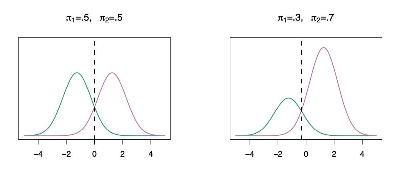
The dashed line is called the Bayes decision boundary.
When the priors are different, we take them into account as well, and compare \(\pi_{k}\)\(f_{k}(x)\). On the right, we favor the light purple class — the decision boundary has shifted to the left.
Discriminant Analysis
LDA improves prediction by accounting for the normally distributed x (continuous).
Bayesian decision boundary
LDA decision boundary
Why not linear regression?
Discriminant Analysis
Linear discriminant analysis is an alternative (and better) method:
-
when the classes are well-separated in multiple-class classification, the parameter estimates for the logistic regression model are surprisingly unstable.
-
If N is small and the distribution of the predictors X is approximately normal in each of the classes, LDA is more stable.
Discriminant Analysis
Linear discriminant analysis
-
Dependent variable: categorical
-
Predictor: continuous + normally distributed
Linear Discriminant Analysis
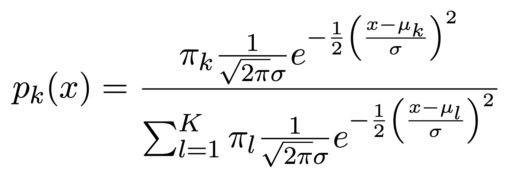
When p=1, The Gaussian density has the form:
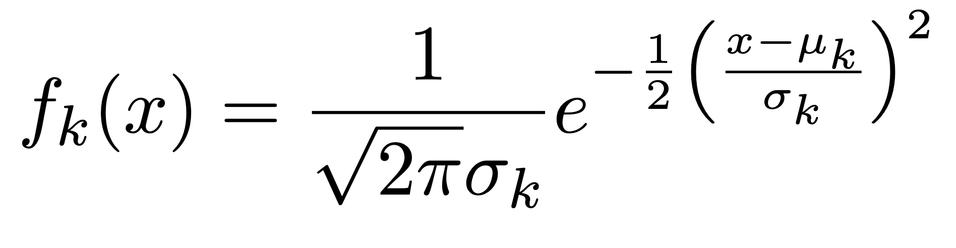
Here \(\mu_{k}\) is the mean, and \(\sigma_{k}^{2}\) the variance (in class k). We will assume that all the \(\sigma_{k}\)=\(\sigma\)are the same. Plugging this into Bayes formula, we get a rather complex expression for \(p_{k}(x)\)=\(Pr(Y=k|X=x)\):
Bayes Theorem
Who is Bayes?

An 18th century English minister who also presented himself as statisticians and philosopher.
His work never was well known until his friend Richard Price found Bayes' notes on conditional probability and got them published.
Lesson to learn: don't tell your friend where you hide your unpublished papers.
~1701-1761
Bayes Theorem
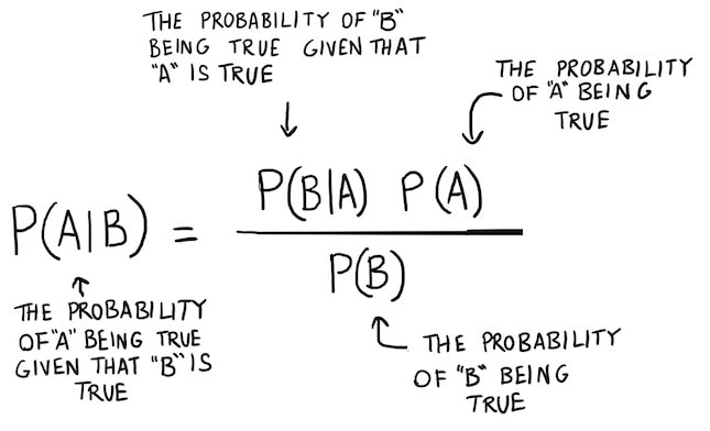
The concept of conditional probability:
Conditional probability is the probability of an event happening, given that it has some relationship to one or more other events.
$$ P(A \mid B) = \frac{P(B \mid A) \, P(A)}{P(B)} $$
To read it, the probability of A given B.
$$ P(A \mid B) = \frac{P(B \mid A) \, P(A)}{P(A)P(B \mid A)+P(\bar{A})P(B \mid \bar{A})} $$
Bayes Theorem
Source: https://www.bayestheorem.net
Bayes Theorem
A prior probability is an initial probability value originally obtained before any
additional information is obtained.
A posterior probability is a probability value that has been revised by using additional
information that is later obtained.
Bayes Theorem
-
The events must be disjoint (with no overlapping).
-
The events must be exhaustive, which means that they combine to include all possibilities
Bayes Theorem
The concept of conditional probability:
Conditional probability is the probability of an event happening, given that it has some relationship to one or more other events.
LDA vs. Logistic regression
LDA assumes that the observations are drawn from a Gaussian distribution with a common covariance matrix in each class, and so can provide some improvements over logistic regression when this assumption approximately holds.
Conversely, logistic regression can outperform LDA if these Gaussian assumptions are not met.
Classification methods
-
Logistic regression is very popular for classification, especially when K = 2.
-
LDA is useful when n is small, or the classes are well separated, and Gaussian assumptions are reasonable. Also when K > 2.
Linear Discriminant Analysis for p >1
Two multivariate Gaussian density functions are shown, with p = 2. Left: The two predictors are uncorrelated. Right: The two variables have a correlation of 0.7.
Linear Discriminant Analysis for p >1
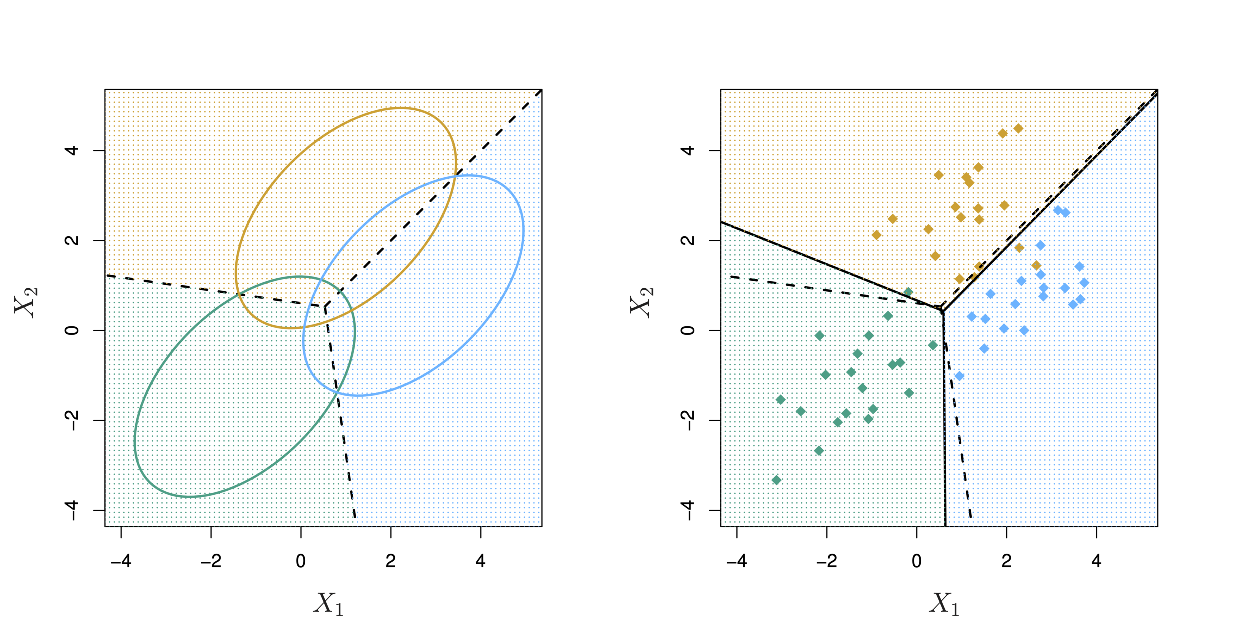
LDA with three classes with observations from a multivariate Gaussian distribution(p = 2), with a class-specific mean vector and a common covariance matrix. Left: Ellipses contain 95 % of the probability for each of the three classes. The dashed lines are the Bayes decision boundaries. Right: 20 observations were generated from each class, and the corresponding LDA decision boundaries are indicated using solid black lines.
Sensitivity and Specificity
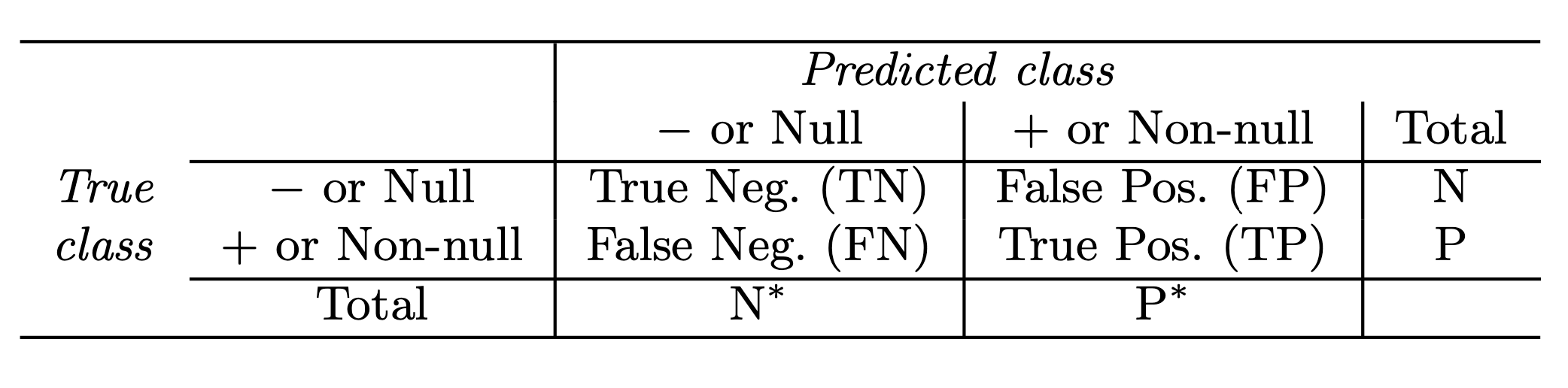
Sensitivity and Specificity

The Receiver Operating Characteristics (ROC) curve display the overall performance of a classifier, summarized over all possible thresholds, is given by the area under the (ROC) curve (AUC). An ideal ROC curve will hug the top left corner, so the larger the AUC the better the classifier.
Confusion matrix: Default data
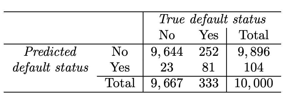
Correct
Incorrect
LDA error: (23+252)/10,000=2.75%
Yet, what matters is how many who actually defaulted were predicted?
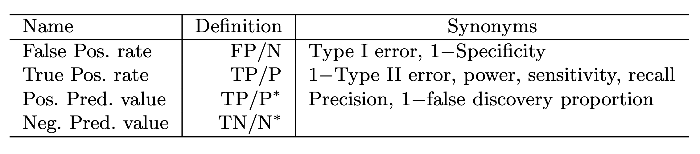
Sensitivity and Specificity
-
Sensitivity is the percentage of true defaulters that are identified (81/333=24.3 % in this case).
-
Specificity is the percentage of non-defaulters that are correctly identified ( (1 − 23/9,667) × 100 = 99.8 %.)
-
Tree-based methods for regression and classification involve stratifying or segmenting the predictor space into a number of simple regions.
-
The set of splitting rules used to segment the predictor space can be summarized in a tree known as decision-tree.
Tree-based methods
-
Tree-based methods are simple and useful for interpretation.
-
However they typically are not competitive with the best supervised learning approaches in terms of prediction accuracy.
-
Methods such as bagging, random forests, and boosting grow multiple trees which are then combined to yield a single consensus prediction.
-
Combining a large number of trees can improve prediction accuracy but at the expense of interpretation.
Tree-based methods
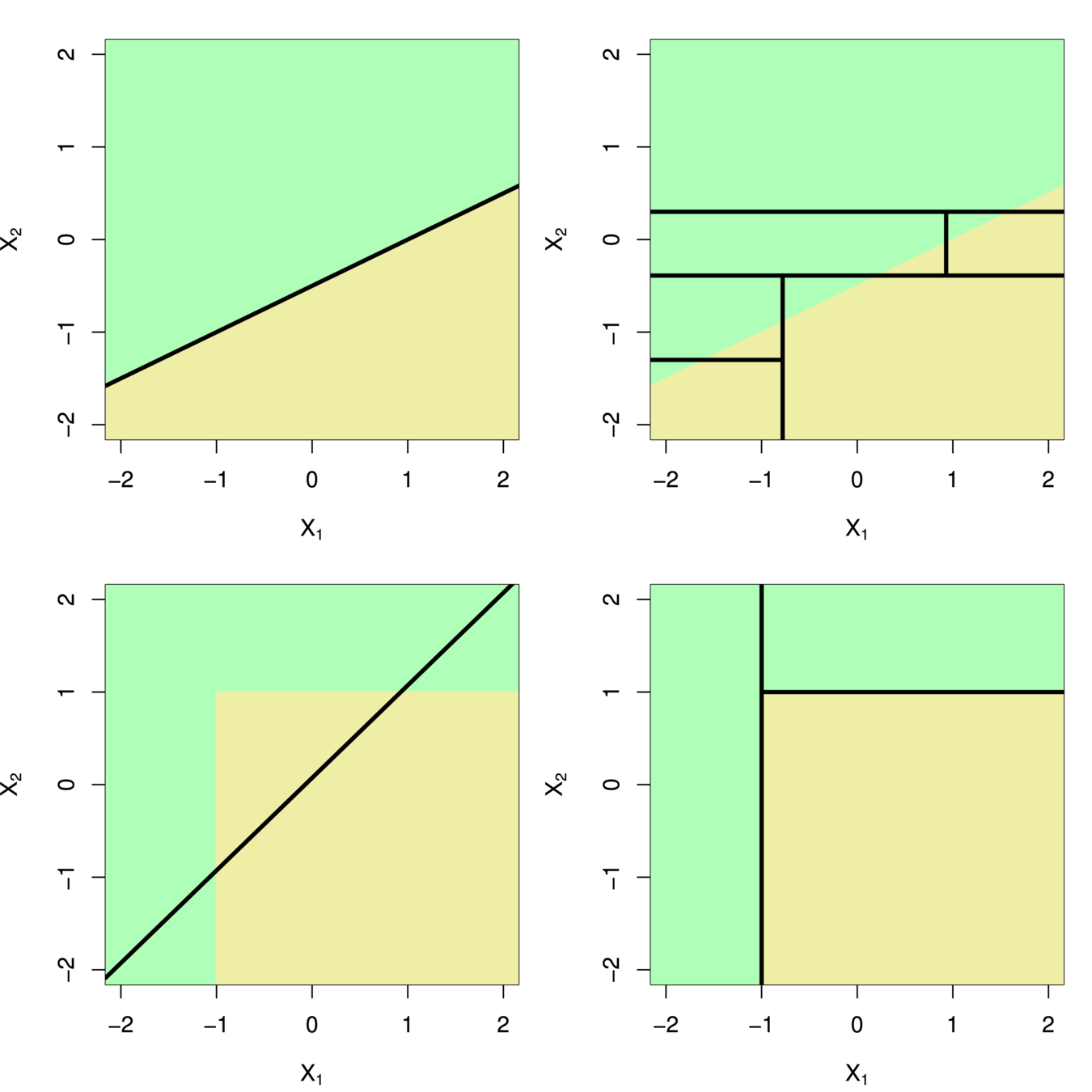
Tree-based methods
A partition of two-dimensional feature space that could not result from recursive binary splitting.
A perspective plot of the prediction surface corresponding to that tree.
A tree corresponding to the partition in the top right panel.
The output of recursive binary splitting on a two-dimensional example.
Decision Trees
-
One way to make predictions in a regression problem is to divide the predictor space (i.e. all the possible values for for \(X_1,X_2,…,X_p)\) into distinct regions, say \(R_1, R_2,…,R_k\)
-
Then for every \(X\) that falls in a particular region (say \(R_j\)) we make the same prediction,
-
Predictor space: set of possible values of \(X_1, X_2,...,X_i\)
-
Divide feature space into \(J\) distinct and non-overlapping regions, \(R_1, R_2,..., R_J\)
-
Predict by mean of observations in every region \(R_j\)
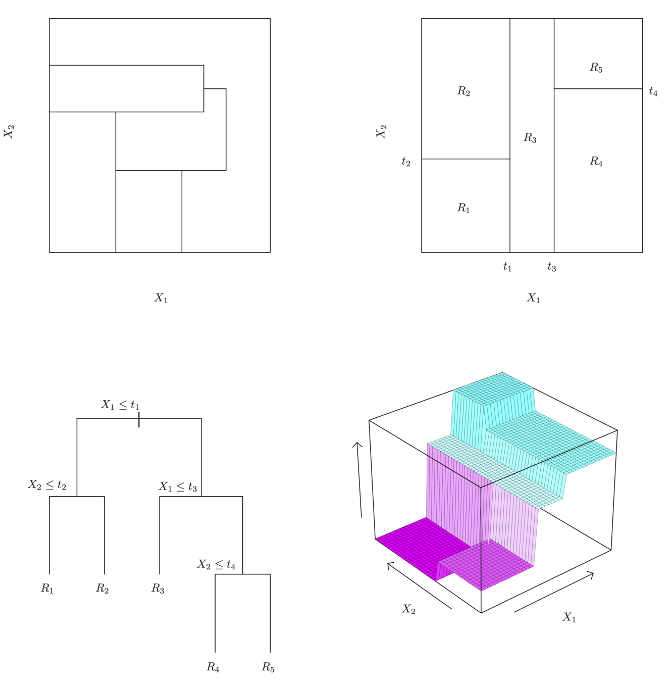
Tree-building process
Splitting the X Variables
-
Generally we create the partitions by iteratively splitting one of the X variables into two regions
\(t_3\)
\(X_1\)
\(X_2\)
- First split on
\(X_1=t_1\) - If \(X_1<t_1\), split on\(X_2=t_2\)
- If \(X_1>t_1\), split on \(X_1=t_3\)
- If \(X_1>t_3\), split on \(X_2=t_4\)
\(t_1\)
\(t_2\)
\(t_4\)
\(R_1\)
\(R_2\)
\(R_3\)
\(R_5\)
\(R_4\)
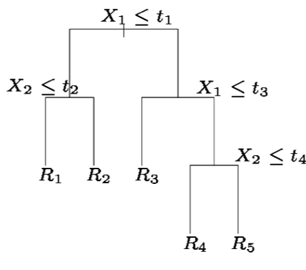
Splitting the X Variables
- When we create partitions this way we can always represent them using a tree structure.
- This provides a very simple way to explain the model to a non-expert.
-
color-coded from low (blue, green) to high (yellow,red)
Baseball salary data

Baseball Salary data
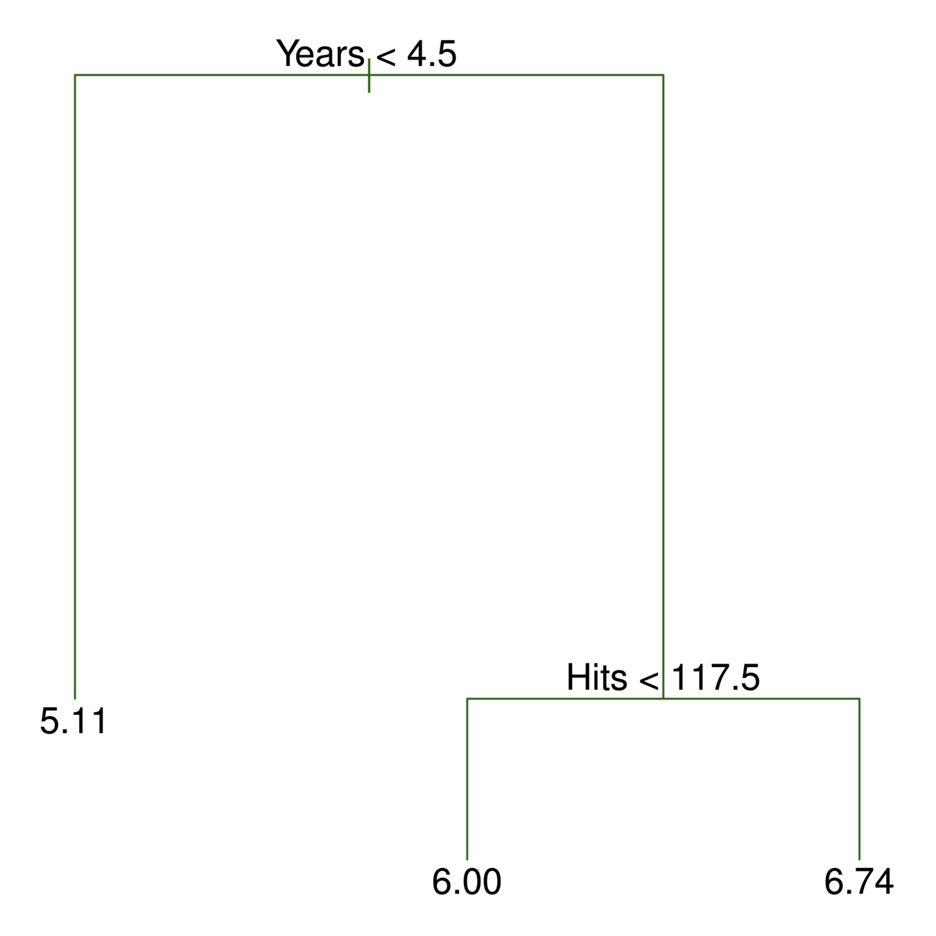
-
color-coded from low (blue, green) to high (yellow,red)
Baseball salary data
117.5
4.5
Here we have two predictors and three distinct regions
-
Decision trees are typically drawn upside down, in the sense that the leaves are at the bottom of the tree.
-
The points along the tree where the predictor space is split are referred to as internal nodes
-
e.g. Years<4.5 and Hits<117.5.
-
Terminal nodes are at end of branch/leaves, which is more meaningful for interpretation
Terminology for Trees
-
A classification tree is very similar to a regression tree except that we try to make a prediction for a categorical rather than continuous Y.
-
For each region (or node) we predict the most common category among the training data within that region.
The tree is grown (i.e. the splits are chosen) in exactly the same way as with a regression tree except that minimizing MSE no longer makes sense. -
There are several possible different criteria to use such as the “gini index” and “cross-entropy” but the easiest one to think about is to minimize the error rate.
Classification Tree
-
A large tree (i.e. one with many terminal nodes) may tend to over fit the training data in a similar way to neural networks without a weight decay.
-
Generally, we can improve accuracy by “pruning” the tree i.e. cutting off some of the terminal nodes.
-
How do we know how far back to prune the tree? We use cross validation to see which tree has the lowest error rate.
Tree Pruning
Baseball Players’ Salaries
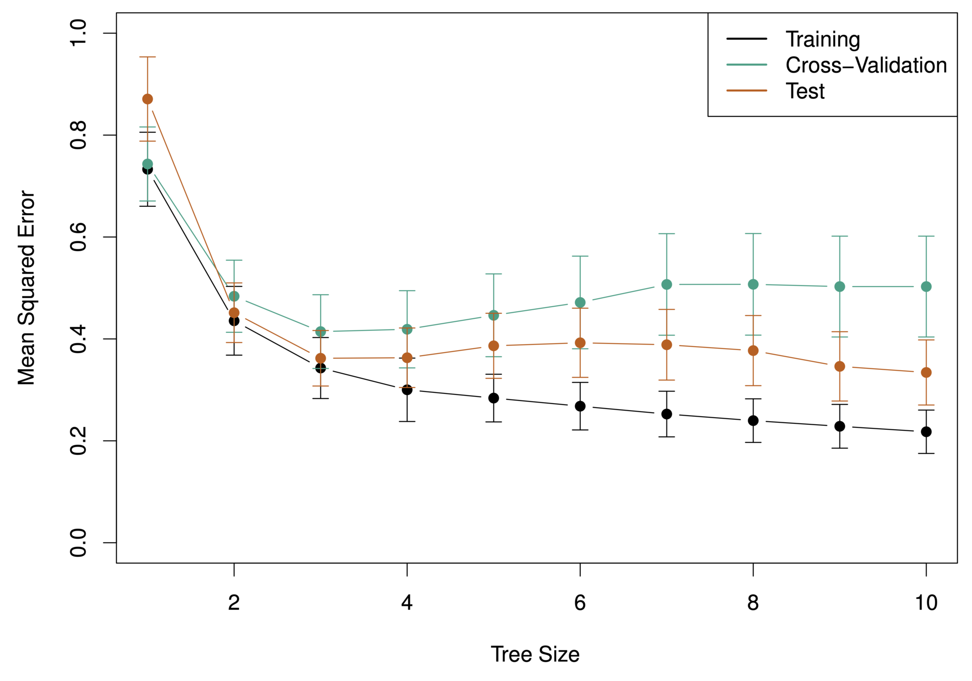
What tree size do we use?
-
If the relationship between the predictors and response is linear, then classical linear models such as linear regression would outperform regression trees
-
On the other hand, if the relationship between the predictors is non-linear, then decision trees would outperform classical approaches
Trees vs. Linear Models
-
High variance!
-
If we randomly split the training data into 2 parts, and fit decision trees on both parts, the results could be quite different
Issues
Decision Trees
| Good | Not so good |
|---|---|
| Highly interpretable (even better than regression) | Prediction Accuracy |
| Plotable | High variance |
| for qualitative predictors (without create dummy variables) | |
| For both regression and classification |
-
Bootstrap: Resampling of the observed dataset (random sampling with replacement from the original dataset and of equal size)
Bagging
(Bootstrap aggregating).
-
Bagging is an extremely powerful idea based on two things:
-
Averaging: reduces variance!
-
Bootstrapping: plenty of training datasets!
-
Bagging
(Bootstrap aggregating).
-
Why does averaging reduces variance?
-
Averaging a set of observations reduces variance.
-
Given a set of \(n\) independent observations \(Z_1, Z_2, …, Z_n\), each with variance, the variance \(\sigma_2\) of the mean \(\bar{x}\) of the observations is given by:
-
Bagging
(Bootstrap aggregating).
$$ \frac{\sigma_2}{n} $$
-
Generate \(B\) different bootstrapped training datasets
-
Train the statistical learning method on each of the \(B\) training datasets, and collect the predictions
-
For prediction:
-
Regression: average all predictions from all \(B\) trees
-
Classification: majority vote among all \(B\) trees
-
Bagging: procedures
-
Construct \(B\) regression trees using \(B\) bootstrapped training datasets
-
Average the resulting predictions
-
These trees are not pruned, so each individual tree has high variance but low bias. Averaging these trees reduces variance, and thus we end up lowering both variance and bias!
Bagging for Regression Trees
-
Construct \(B\) trees using \(B\) bootstrapped training datasets
-
For prediction, there are two approaches:
-
Record the class that each bootstrapped data set predicts and provide an overall prediction to the most commonly occurring one (majority vote).
-
If our classifier produces probability estimates we can just average the probabilities and then predict to the class with the highest probability.
-
Bagging for Classification Trees
Error rates
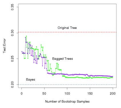
-
Green line represents a simple majority vote approach
-
Purple line corresponds to averaging the probability estimates.
-
Both do far better than a single tree (dashed red) and get close to the Bayes error rate (dashed grey).

Error rates
-
On average, each bagged tree makes use of around two-thirds of the observations.
-
The remaining one-third of the observations not used to fit a given bagged tree are referred to as the out-of-bag (OOB) observations.
-
Predict the response for the \(i^{th}\) observation using each of the trees in which that observation was OOB. This will yield around \(\frac{B}{3}\) predictions for the \(i^{th}\) observation, which we average.
-
This estimate is essentially the Leave One Out (LOO) cross-validation error for bagging, if \(B\) is large
Out-of-Bag (OOB) Error Estimation
-
Bagging typically improves the accuracy over prediction using a single tree, but it is now hard to interpret the model!
-
We have hundreds of trees, and it is no longer clear which variables are most important to the procedure
Thus bagging improves prediction accuracy at the expense of interpretability. -
But, we can still get an overall summary of the importance of each predictor using Relative Influence Plots
Variable Importance Measure
-
Relative Influence Plots give a score for each variable.
-
These scores represents the decrease in MSE when splitting on a particular variable
-
A number close to zero indicates the variable is not important and could be dropped.
-
The larger the score the more influence the variable has.
Relative Influence Plots
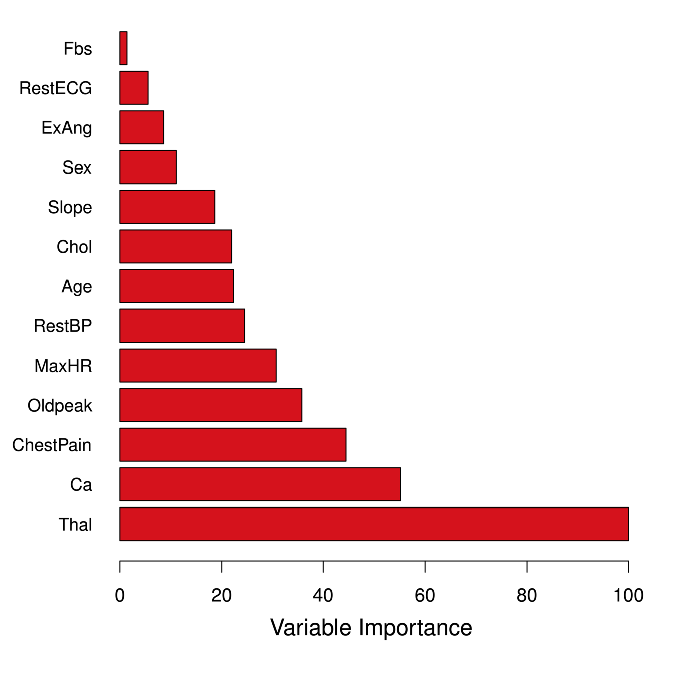
-
Relative Influence Plots give a score for each variable.
-
These scores represents the decrease in MSE when splitting on a particular variable
-
A number close to zero indicates the variable is not important and could be dropped.
-
The larger the score the more influence the variable has.
Relative Influence Plots
- age
- sex
- chest pain type (4 values)
- resting blood pressure
- serum cholestoral in mg/dl
- fasting blood sugar > 120 mg/dl
- resting electrocardiographic results (values 0,1,2)
- maximum heart rate achieved
- exercise induced angina
- oldpeak = ST depression induced by exercise relative to rest
- the slope of the peak exercise ST segment
- number of major vessels (0-3) colored by flourosopy
- thal (Thalassemias): 3 = normal; 6 = fixed defect; 7 = reversable defect
Relative Influence Plots: Heart data
age
sex
chest pain type (4 values)
resting blood pressure
serum cholestoral in mg/dl
fasting blood sugar > 120 mg/dl
resting electrocardiographic results (values 0,1,2)
maximum heart rate achieved
exercise induced angina
oldpeak = ST depression induced by exercise relative to rest
the slope of the peak exercise ST segment
number of major vessels (0-3) colored by flourosopy
thal (Thalassemias): 3 = normal; 6 = fixed defect; 7 = reversable defect
Random Forests
- Why a random sample of \(m\) predictors instead of all \(p\) predictors for splitting?
- Suppose that we have a very strong predictor in the data set along with a number of other moderately strong predictor, then in the collection of bagged trees, most or all of them will use the very strong predictor for the first split!
- All bagged trees will look similar. Hence all the predictions from the bagged trees will be highly correlated
- Averaging many highly correlated quantities does not lead to a large variance reduction
- Random forests “de-correlates” the bagged trees leading to more reduction in variance
Random Forests
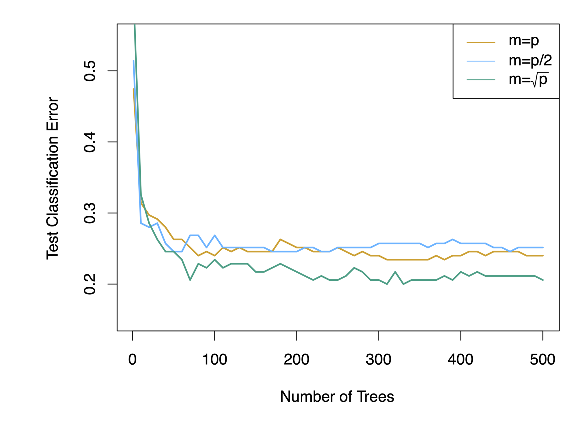
When \(m = p\), this is simply the bagging model.
Random Forests
-
Building on the idea of bagging, random forest provides an improvement because it de-correlates the trees
-
Procedures:
-
Build a number of decision trees on bootstrapped training sample
-
When building the trees, each time a split in a tree is considered
-
a random sample of \(m\) predictors is chosen as split candidates from the full set of \(p\) predictors (Usually \(m\approx\sqrt{p}\) )
-