Gentle Introduction to Machine Learning
Karl Ho
School of Economic, Political and Policy Sciences
University of Texas at Dallas
Workshop prepared for International Society for Data Science and Analytics (ISDSA) Annual Meeting, Notre Dame University, June 2nd, 2022.
Unsupervised Learning
Unsupervised Learning
-
No response variable \(Y\)
-
Not interested in prediction
-
The goal is to discover interesting patterns about the measurements on \(X_{1}\), \(X_{2}\), . . . , \(X_{p}\)
-
Any subgroups among the variables or among the observations?
-
Principal components analysis
-
Clustering
-
Supervised vs. Unsupervised Learning
-
Supervised Learning: both X and Y are known
-
Unsupervised Learning: only X

Challenge
Unsupervised learning is more subjective than supervised learning, as there is no simple prediction of a response.
-
But unsupervised learning is growing popular in fields like:
Medicine: grouping cancer patients by gene expression measurements;
Marketing: grouping shoppers by browsing and purchase histories;
Entertainment: movies grouped by movie viewer ratings.
Principal Components Analysis
-
Principal Components Analysis (PCA) produces a low-dimensional representation of a dataset. It finds a sequence of linear combinations of the variables that have maximal variance, and are mutually uncorrelated.
-
Apart from producing derived variables for use in supervised learning problems, PCA also serves as a tool for data visualization.
Principal Components Analysis
-
The first principal component of a set of features
\(X_1, X_2, . . . , X_p\) is the normalized linear combination of the features:
-
that has the largest variance. By normalized, we mean that
\(\sum_{j=1}^p\phi_{j1}^2 = 1\). -
The elements \(\phi_{11}, . . . , \phi_{p1}\) are the loadings of the first principal component; together, the loadings make up
the principal component loading vector, \(\phi_1 = (\phi_{11} \phi_{21} ... \phi_{p1})^T\) . -
We constrain the loadings so that their sum of squares is equal to one, since otherwise setting these elements to be arbitrarily large in absolute value could result in an arbitrarily large variance.
\(Z_1 = \phi_{11}X_1 +\phi_{21}X_2 +...+\phi_{p1}X_p\)
Principal Components Analysis
-
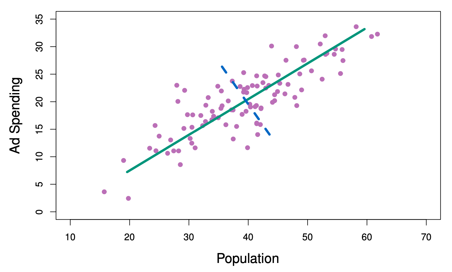
The population size (pop) and ad spending (ad) for 100 different cities are shown as purple circles. The green solid line indicates the first principal component direction, and the blue dashed line indicates the second principal component directio
Computation of Principal Components
-
Suppose we have a \(n×p\) data set \(X\). Since we are only interested in variance, we assume that each of the variables in \(X\) has been centered to have mean zero (that is, the column means of \(X\)are zero).
-
We then look for the linear combination of the sample feature values of the form
-
for \(i = 1, . . . , n\) that has largest sample variance, subject to
the constraint that \(\sum^p_{j=1} \phi^2_{j1} = 1\). -
Since each of the \(x_{ij}\) has mean zero, then so does \(z_{i1}\) (for any values of \(\phi_{j1}\)). Hence the sample variance of the \(z_{i1}\) can be written as \(\frac{1}{n}\sum^n_{i=1}z_{i1}^2\).
\(Z_{i1} = \phi_{11}X_{i1} +\phi_{21}X_{i2} +...+\phi_{p1}X_{ip}\)
(1)
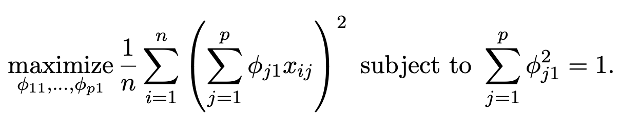
Computation of Principal Components
-
Plugging in (1) the first principal component loading vector solves the optimization problem
-
This problem can be solved via a singular-value decomposition of the matrix \(X\), a standard technique in linear algebra.
-
We refer to \(Z_1\) as the first principal component, with realized values \(z_{11}, . . . , z_{n1}\)
Geometry of PCA
-
The loading vector \(\phi_1\) with elements \(\phi_{11}, \phi_{21},...,\phi_{p1}\) defines a direction in feature space along which the data vary the most.
-
If we project the \(n\) data points \(x_1,...,x_n\) onto this direction, the projected values are the principal component scores \(z_{11},...,z_{n1}\) themselves.
Further principal components
-
The second principal component is the linear combination of \(X_1, . . . , X_p\) that has maximal variance among all linear combinations that are uncorrelated with \(Z_1\).
-
The second principal component scores \(z_{12}, z_{22},..., z_{n2}\) take the form:
\(z{i2} = \phi_{12}x_{i1} + \phi_{22}x_{i2} +...+ \phi_{p2}x_{ip}\),
where \(\phi_2\) is the second principal component loading vector, with elements \(\phi_{12}, \phi_{22}, . . . , \phi_{p2}\).
Further principal components
-
It turns out that constraining \(Z_2\) to be uncorrelated with \(Z_1\) is equivalent to constraining the direction \(\phi_2\) to be orthogonal (perpendicular) to the direction \(\phi_1\). And so on.
-
The principal component directions \(\phi_1\),\(\phi_2\), \(\phi_3\), . . . are the ordered sequence of right singular vectors of the matrix \(X\), and the variances of the components are \(\frac{1}{n}\) times the squares of the singular values. There are at most
\(min(n − 1, p)\) principal components.
Illustration: US Arrests
-
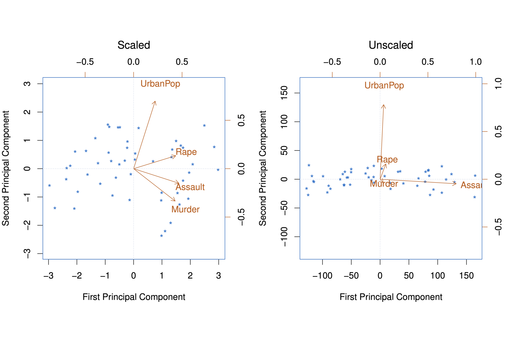
The first two principal components for the USArrests data.
-
The black state names represent the scores for the first two principal components.
-
The red arrows indicate the first two principal component loading vectors (with axes on the top and right). For example, the loading for Rape on the first component is 0.54, and its loading on the second principal component 0.17 [the word Rape is centered at the point (0.54, 0.17)]. (Note scale difference in plot)

                PC1        PC2        PC3         PC4
Murder   -0.5358995  0.4181809 -0.3412327  0.64922780
Assault  -0.5831836  0.1879856 -0.2681484 -0.74340748
UrbanPop -0.2781909 -0.8728062 -0.3780158  0.13387773
Rape     -0.5434321 -0.1673186  0.8177779  0.08902432
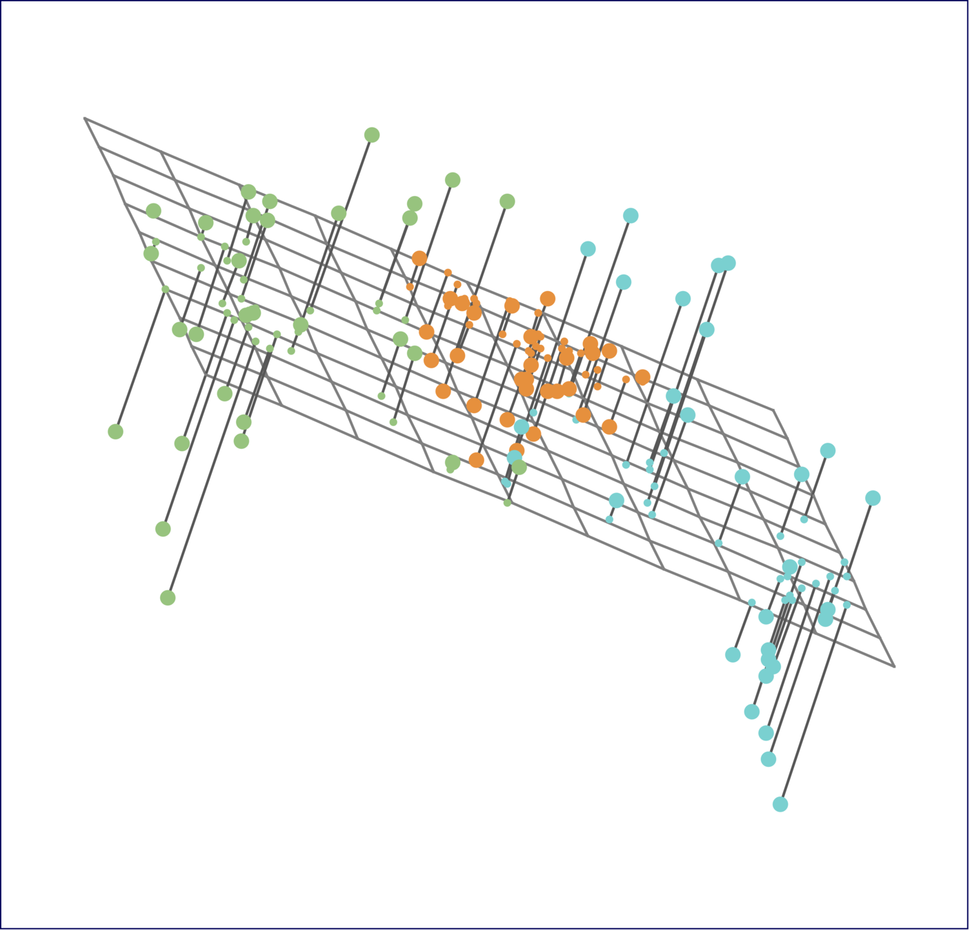
PCA find the hyperplane closest to the observations
-
The first principal component loading vector has a very special property: it defines the line in \(p\)-dimensional space that is closest to the \(n\) observations (using average squared Euclidean distance as a measure of closeness)
-
The notion of principal components as the dimensions that are closest to the \(n\) observations extends beyond just the first principal component.
-
For instance, the first two principal components of a data set span the plane that is closest to the \(n\) observations, in terms of average squared Euclidean distance.
Scaling of the variables matters
-
If the variables are in different units, scaling each to have standard deviation equal to one is recommended.
-
If they are in the same units, you might or might not scale the variables.
Elbow Method
-
The elbow method looks at the percentage of variance explained as a function of the number of clusters,
-
Choose a number of clusters so that adding another cluster doesn’t give much better modeling of the data.

Clustering
-
Clustering refers to a set of techniques for finding subgroups, or clusters, in a data set.
-
A good clustering is one when the observations within a group are similar but between groups are very different
-
For example, suppose we collect p measurements on each of n breast cancer patients. There may be different unknown types of cancer which we could discover by clustering the data
Different Clustering Methods
-
There are many different types of clustering methods
-
Two most commonly used approaches:
-
K-Means Clustering
-
Hierarchical Clustering
-
K-Means Clustering
-
To perform K-means clustering, one must first specify the desired number of clusters K
-
Then the K-means algorithm will assign each observation to exactly one of the K clusters

How does K-Means work?
We would like to partition that data set into K clusters:
- Each observation belong to at least one of the K clusters
-
The clusters are non-overlapping, i.e. no observation belongs to more than one cluster
-
The objective is to have a minimal “within-cluster-variation”, i.e. the elements within a cluster should be as similar as possible
-
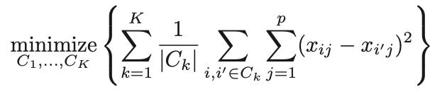
One way of achieving this is to minimize the sum of all the pair-wise squared Euclidean distances between the observations in each cluster.
\(C_1,...,C_K\)
K-Means Algorithm
- Step 1: Randomly assign each observation to one of K clusters
- Step 2: Iterate until the cluster assignments stop changing:
- For each of the K clusters, compute the cluster centroid. The \(k^{th}\) cluster centroid if the mean of the observations assigned to the \(k^{th}\) cluster
- Assign each observation to the cluster whose centroid is closest (where “closest” is defined using Euclidean distance.
K-Means Algorithm
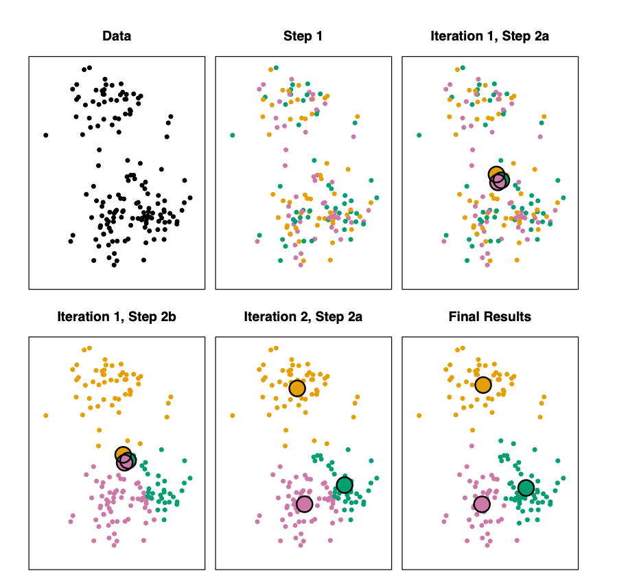
K-Means Algorithm
Step 1: random assignment of points to k groups
Iteration 1 Step 2a:
Compute cluster centroids
Iteration 1 Step 2b:
Assign points to closest cluster center
Iteration 2 Step 2a:
Compute new cluster centroids
Stop at k center points where there's no further change.
K-Means Cluster: Iris data

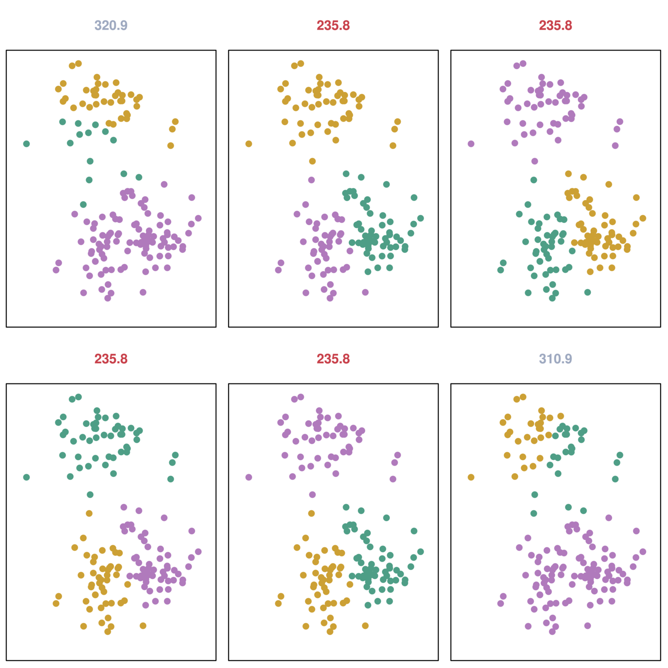
Different starting values
Different starting values
- K-means clustering performed six times on the data with K = 3, each time with a different random assignment of the observations.
- Three different local optima were obtained, one of which resulted in a smaller value of the objective and provides better separation between the clusters.
- Those labeled in red all achieved the same best solution, with an objective value of 235.8
Hierarchical Clustering
-
K-Means clustering requires choosing the number of clusters.
-
An alternative is Hierarchical Clustering which does not require that we commit to a particular choice of \(K\).
-
Hierarchical Clustering has an advantage that it produces a tree-based representation of the observations: Dendrogram
-
A dendrogram is built starting from the leaves and combining clusters up to the trunk.
Dendrograms
-
First join closest points (5 and 7)
-
Height of fusing/merging (on vertical axis) indicates how similar the points are
-
After the points are fused they are treated as a single observation and the algorithm continues
Interpretation
-
Each “leaf” of the dendogram represents one of the 45 observations
-
At the bottom of the dendogram, each observation is a distinct leaf. However, as we move up the tree, some leaves begin to fuse. These correspond to observations that are similar to each other.
-
As we move higher up the tree, an increasing number of observations have fused. The earlier (lower in the tree) two observations fuse, the more similar they are to each other.
-
Observations that fuse later are quite different
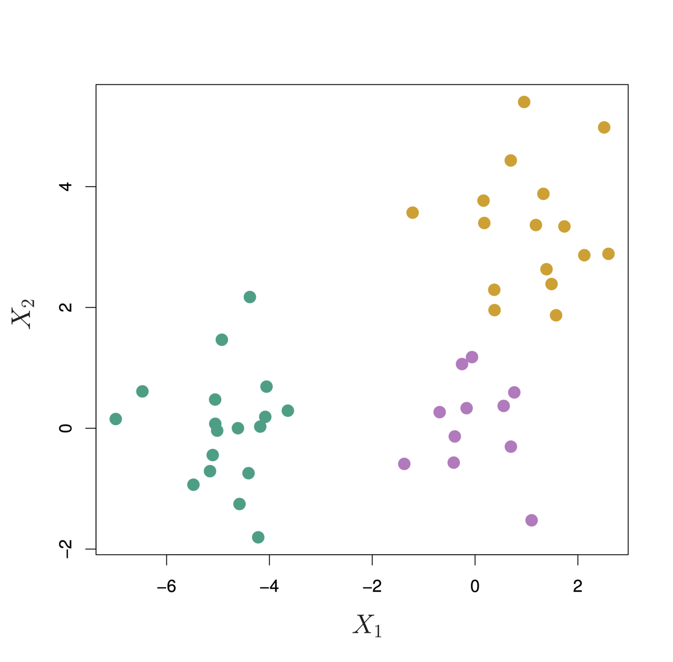
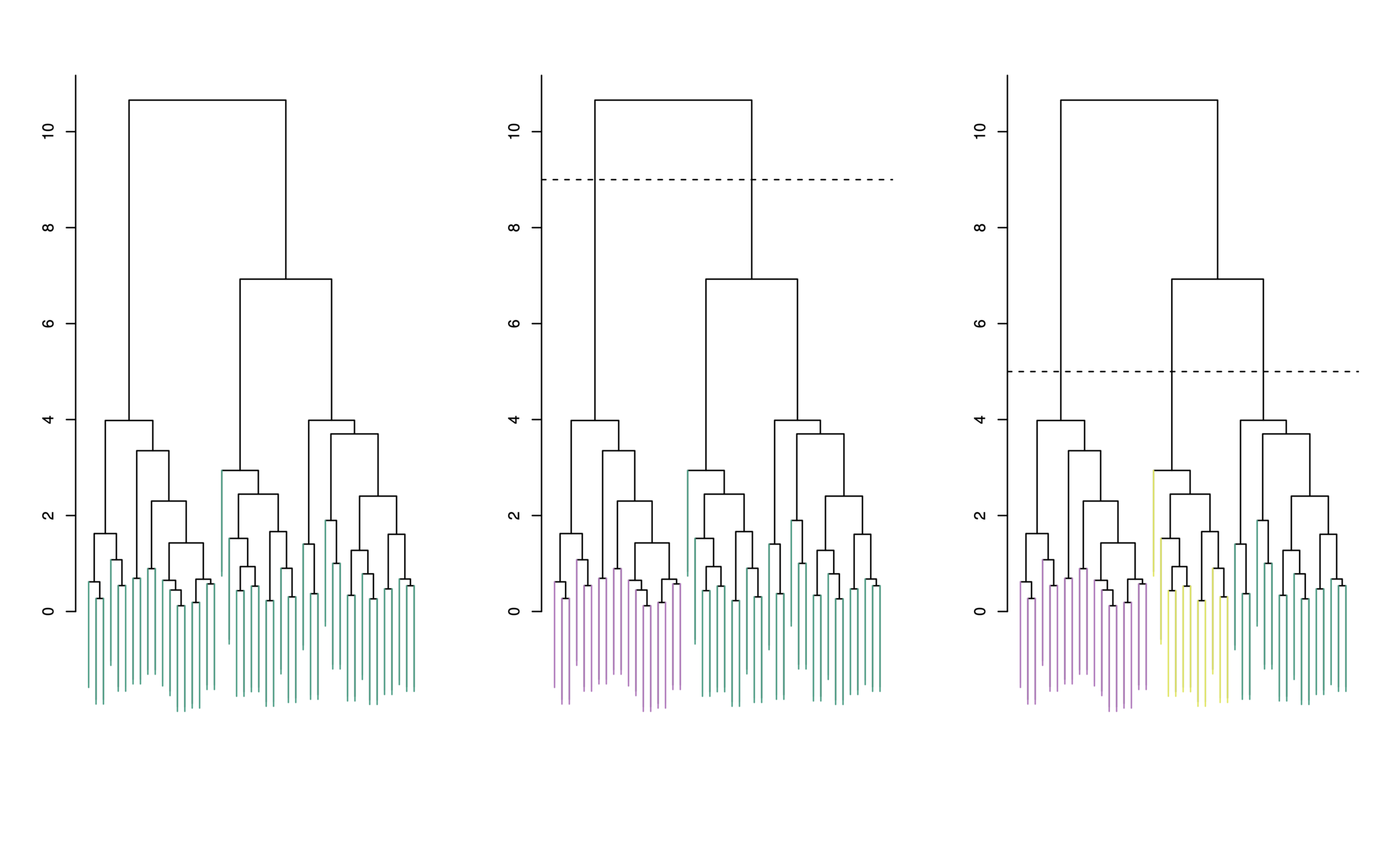
Choosing Clusters
-
To choose clusters we draw lines across the dendrogram
-
We can form any number of clusters depending on where we draw the break point.
One cluster
Two clusters
Three clusters
Agglomerative Approach
To build the dendrogram:
-
Start with each point as a separate cluster (\(n\) clusters)
-
Calculate a measure of dissimilarity between all points/clusters
-
Fuse two clusters that are most similar so that there are now \(n-1\) clusters
-
Fuse next two most similar clusters so there are now \(n-2\) clusters
-
Continue until there is only 1 cluster
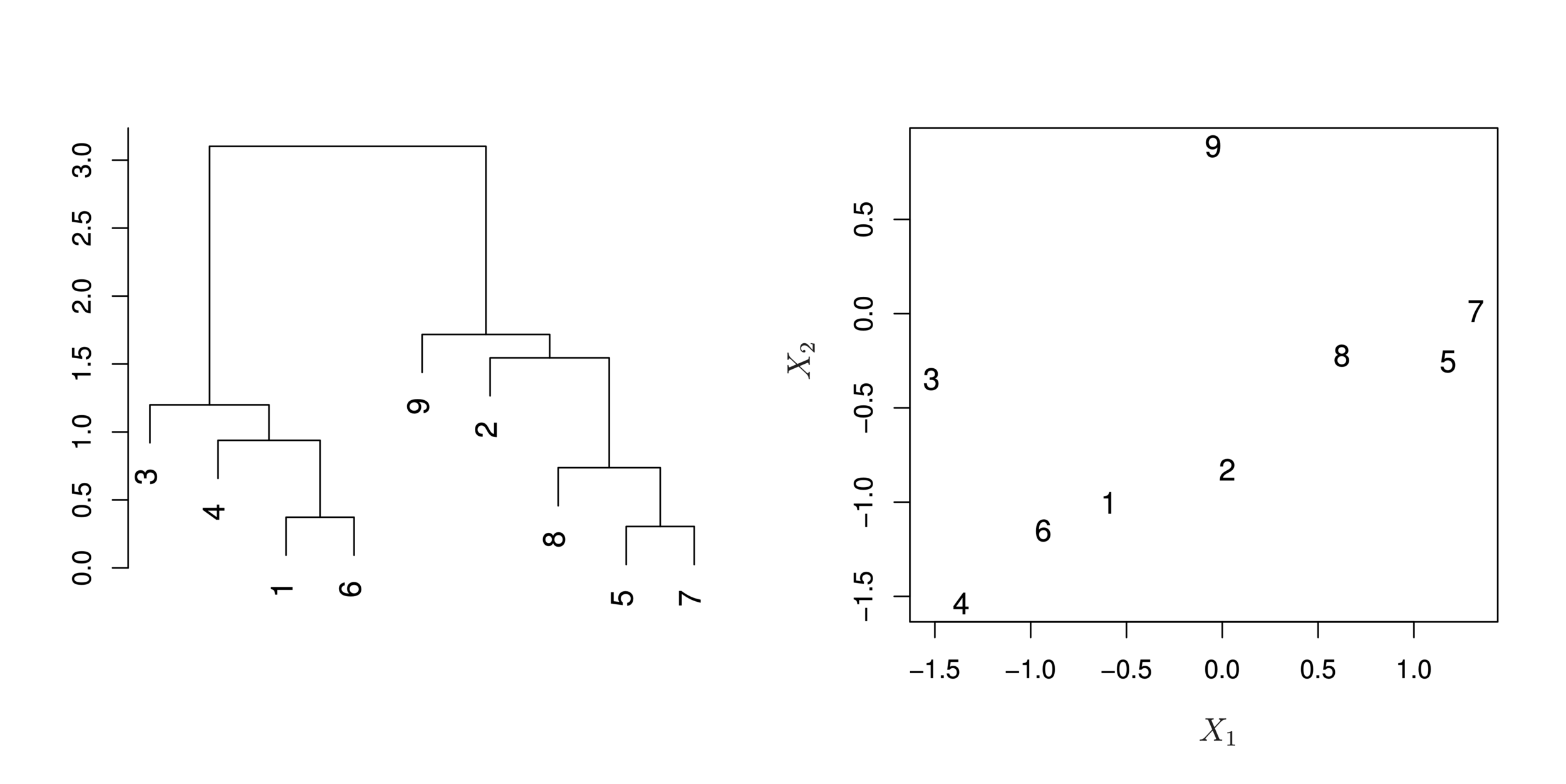
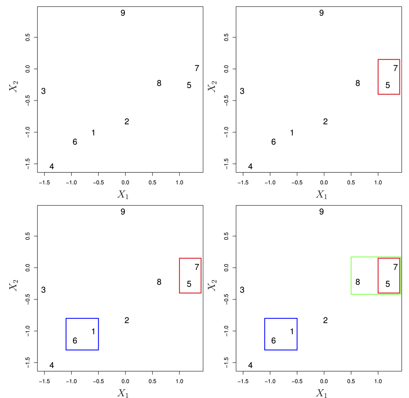
Illustration
- Start with 9 clusters
- Fuse 5 and 7
- Fuse 6 and 1
- Fuse the (5,7) cluster with 8.
- Continue until all observations are fused.
Dissimilarity
- How do we define the dissimilarity, or linkage, between the fused (5,7) cluster and 8?
- There are four options:
- Complete Linkage
- Single Linkage
- Average Linkage
- Centriod Linkage
Linkage Methods: Distance Between Clusters
- Complete Linkage:
- Largest distance between observations
- Single Linkage:
- Smallest distance between observations
- Average Linkage:
- Average distance between observations
- Centroid:
- Distance between centroids of the observations
- Distance between centroids of the observations
Linkage Methods: Distance Between Clusters
|
Complete |
Maximal inter-cluster dissimilarity. Compute all pairwise dissimilarities between the observations in cluster A and the observations in cluster B, and record the largest of these dissimilarities. |
|
Single |
Minimal inter-cluster dissimilarity. Compute all pairwise dissimilarities between the observations in cluster A and the observations in cluster B, and record the smallest of these dissimilarities. |
|
Average |
Mean inter-cluster dissimilarity. Compute all pairwise dissimilarities between the observations in cluster A and the observations in cluster B, and record the average of these dissimilarities. |
|
Centroid |
Dissimilarity between the centroid for cluster A (a mean vector of length p) and the centroid for cluster B. Centroid linkage can result in undesirable inversions. |
Linkage Methods: Distance Between Clusters
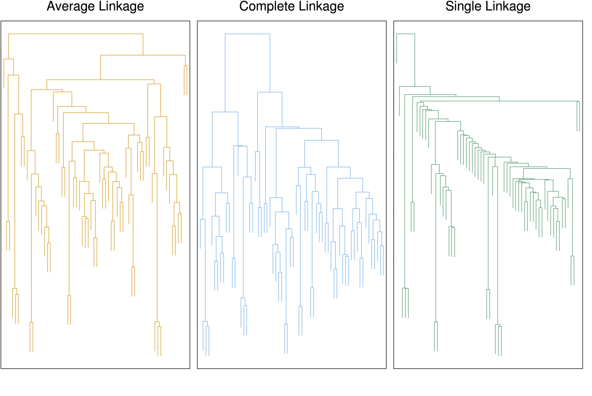
- These dendrograms show three clustering results for the same data
- The only difference is the linkage method but the results are very different
- Complete and average linkage tend to yield evenly sized clusters whereas single linkage tends to yield extended clusters to which single leaves are fused one by one.
Choice of Dissimilarity Measure
-
We have considered using Euclidean distance as the dissimilarity measure
-
An alternative is correlation-based distance which considers
two observations to be similar if their features are highly
correlated. -
This is an unusual use of correlation, which is normally
computed between variables; here it is computed between the observation profiles for each pair of observations.
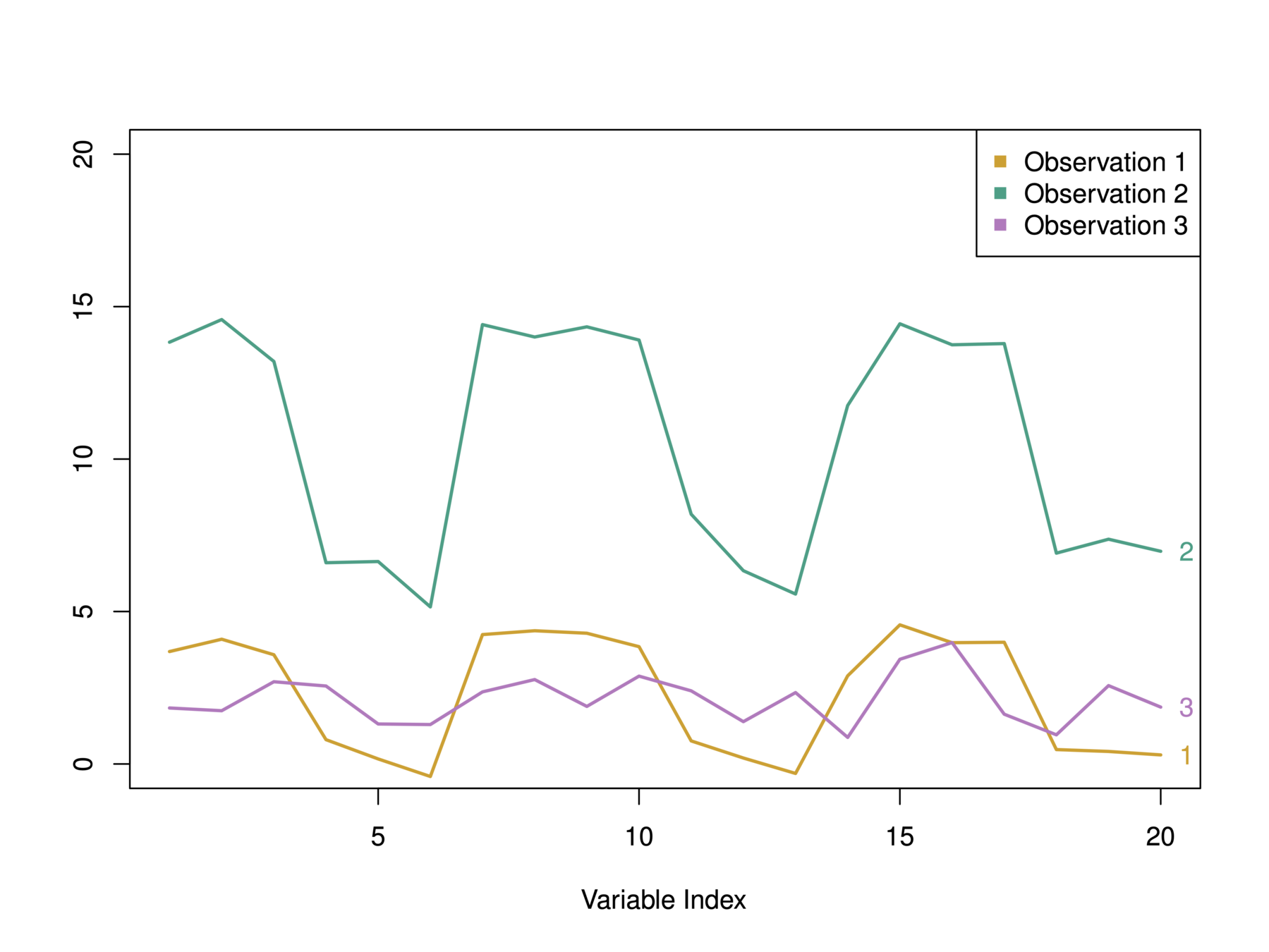
In this example, we have 3 observations and p = 20 variables
In terms of Euclidean distance obs. 1 and 3 are similar. However, obs. 1 and 2 are highly correlated so would be considered similar in terms of correlation measure.
Illustration: Online shopping
-
Suppose we record the number of purchases of each item (columns) for each customer (rows)
-
Using Euclidean distance, customers who have purchases very little will be clustered together
-
Using correlation measure, customers who tend to purchase the same types of products will be clustered together even if the magnitude of their purchase may be quite different
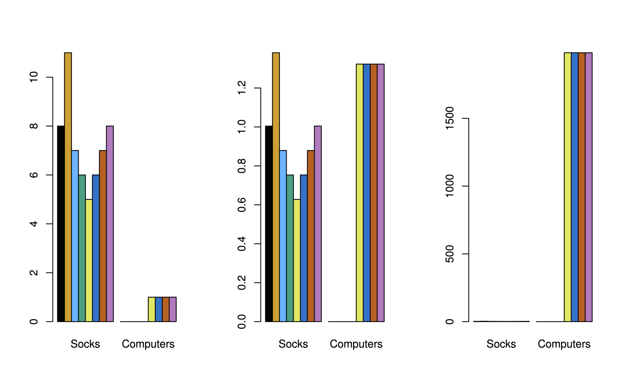
Illustration: Online shopping
-
Consider an online shop that sells two items: socks and computers
-
Left: In terms of quantity, socks have higher weight
-
Center: After standardizing, socks and computers have equal weight
-
Right: In terms of dollar sales, computers have higher weight
-
Quantity
Price
Key decisions in Clustering
-
Should the features first be standardized? i.e. Have the variables centered to have a mean of zero and standard deviation of one.
-
For K-means clustering,
-
How many clusters should be set?
-
-
For Hierarchical Clustering,
-
What dissimilarity measure should be used?
-
What type of linkage should be used?
-
Where should we cut the dendrogram in order to obtain clusters?
-
-
In real world research, try several different choices, and decide on one that is interpretable!
Conclusions
-
Unsupervised learning is important for understanding the variation and grouping structure of a set of unlabeled data, and can be a useful pre-processor for supervised learning
-
It is intrinsically more difficult than supervised learning because there is no gold standard (like an outcome variable) and no single objective (like test set accuracy).
-
It is an active field of research, with many recently developed tools such as self-organizing maps, independent components analysis and spectral clustering.
Deep Learning
Deep learning is a neural-networks technique that organizes the neurons in many more than multi-layer perceptrons. It is in this sense the networks are “deep,” and this is what gave the paradigm its name.
- The top layers of these networks are trained by a supervised learning technique such as the back-propagation of error. By contrast, the task for the lower layers is to create a reasonable set of features. It is conceivable that self-organizing feature maps be used to this end; in reality, more advanced techniques are usually preferred.
- If the number of features is manageable, and if the size of
the training set is limited, then classical approaches will do just as well as deep learning or even better