Learning from DeFi: Would AMMs Improve Equity Trading?
Katya Malinova & Andreas Park
The Economics of Liquidity Provision CDFT, CBER, Uniswap Labs
NYC June 13, 2025

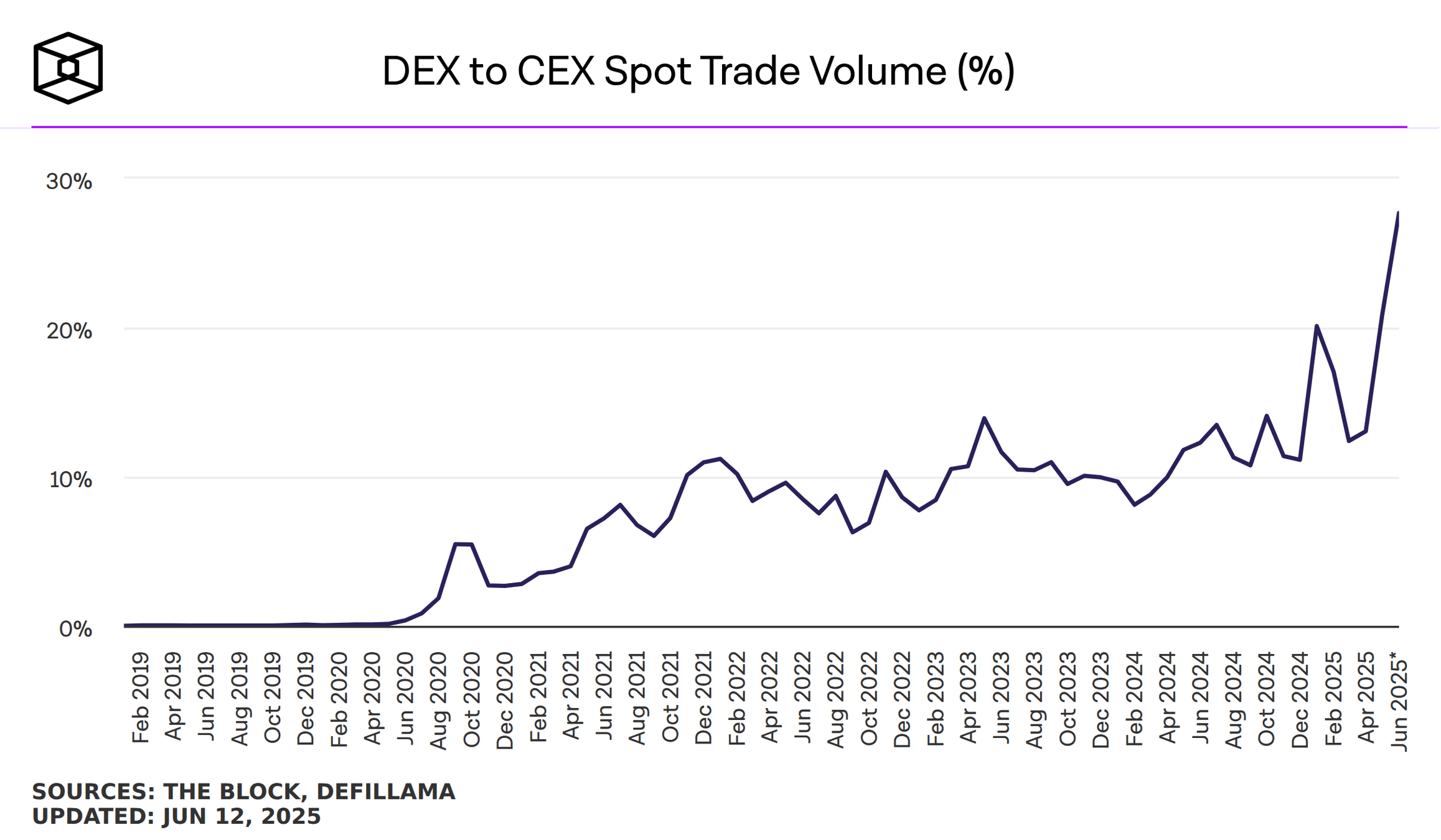
- Blockchain: borderless general purpose value and resource management tool
Preliminaries
- DeFi: financial applications that run on blockchains
- \(\Rightarrow\) brought new ideas and tools
- one new market institution: automated market makers
Quick Recap: Automated Market Makers (AMM)









Liquidity providers
Liquidity demander
Liquidity Pool

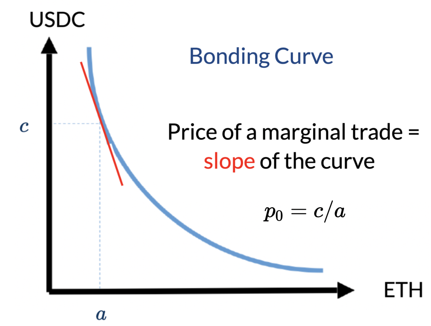
AMM pricing is mechanical:
- determined by the amounts of deposits
- most common:
- constant product
- #USDC \(\times\) #ETH = const
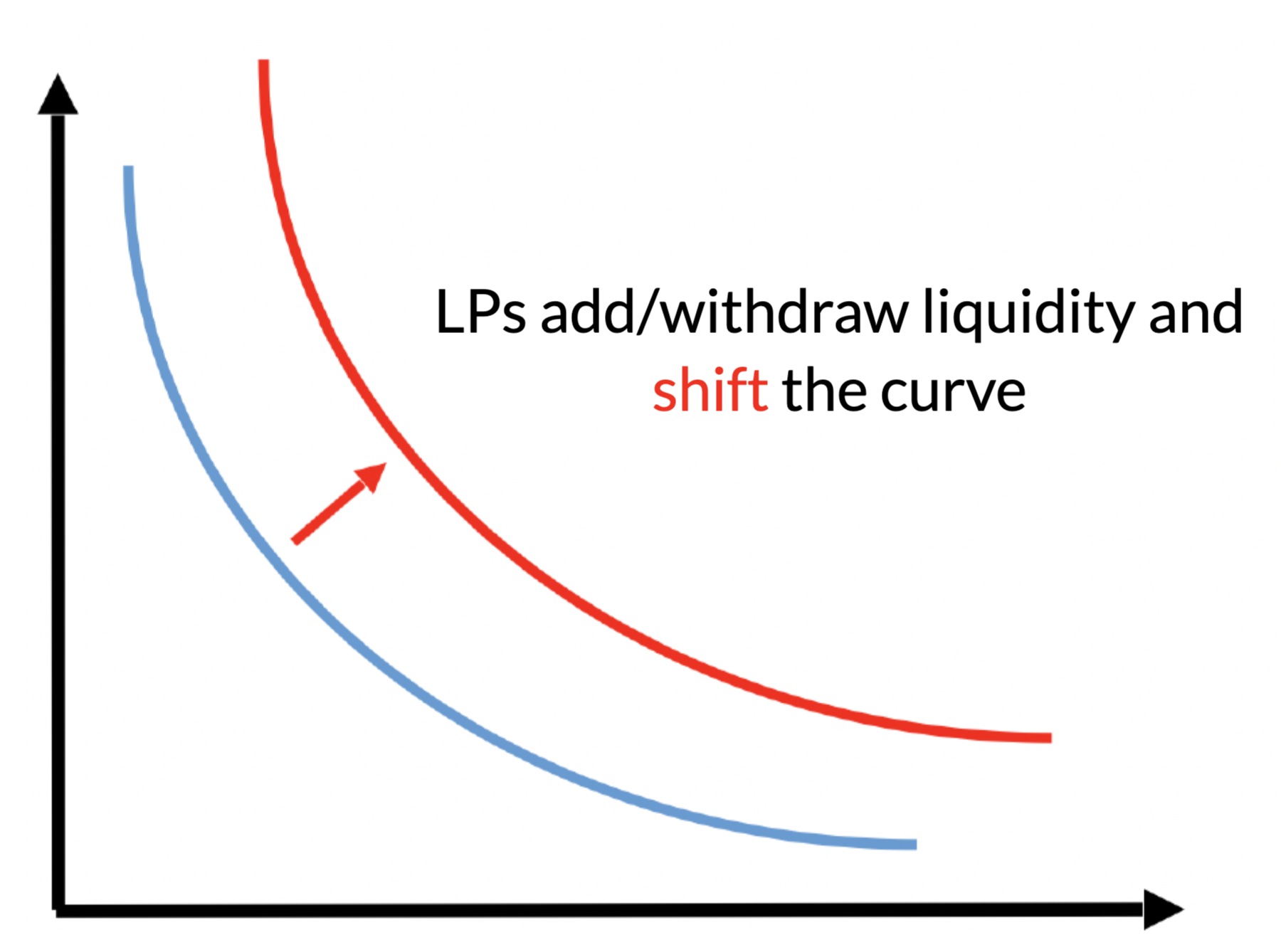
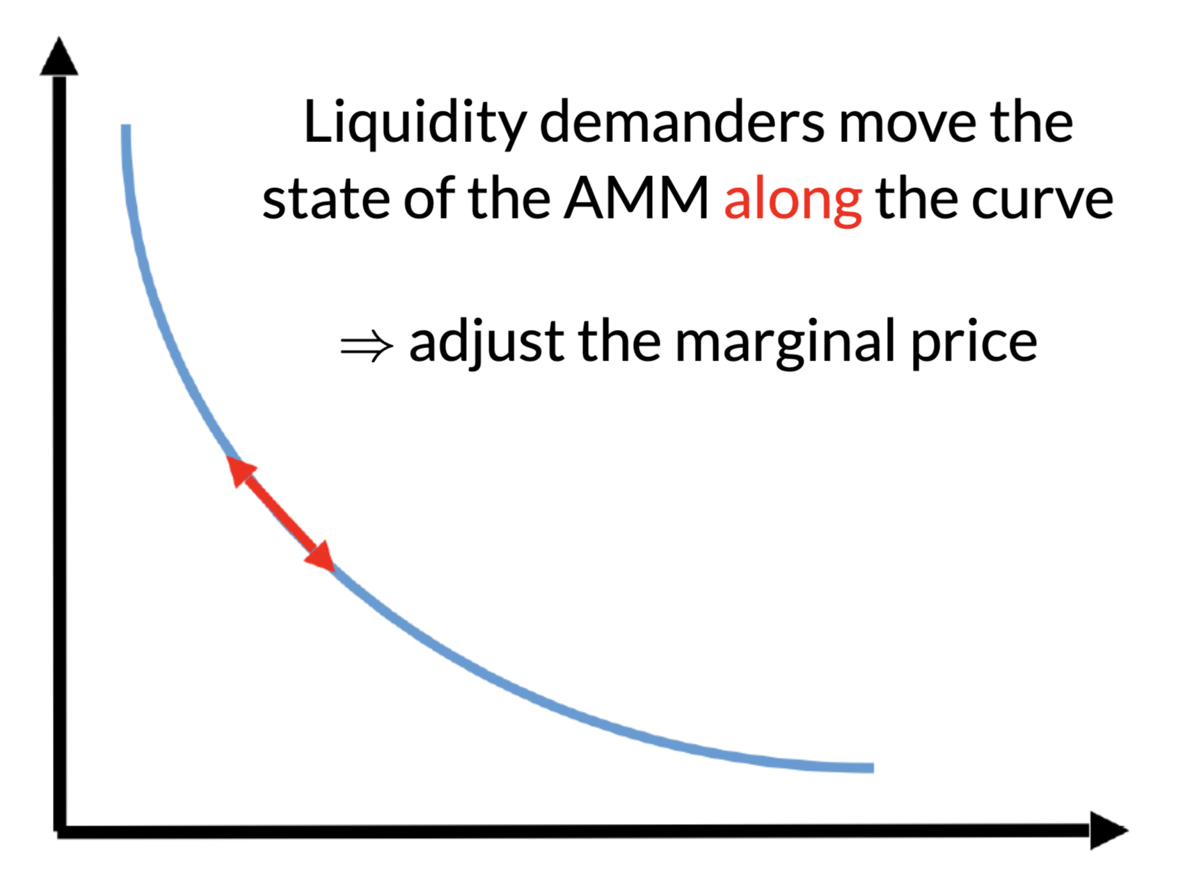
No effect on the marginal price
Key Components
- Our question:
- Can an economically viable AMM be designed for current equity markets?
- Would such an AMM improve current markets?
- Pooling of liquidity!
- Liquidity providers:
- pro-rated
- risk
- trading fee income
- use assets that they own to earn passive (fee) income
- retain exposure to the asset
- pro-rated
- Liquidity demanders:
- predictable price
- continuous\(^*\) trading
- ample liquidity
Existing asset holders, not market makers, do not aim for zero inventory!
Modelling Calibrate-able Liquidity Supply and Demand in an Automated Market Maker
Facts about modelling liquidity provision
- You provide liquidity when the marginal price at the AMM and elsewhere is \(p(t_0)=p.\)
- You make a decision what to do next at \(t_1>t_0\)
- Many things can happen, for instance:
- AMM trades
- price moves in the broader markets
Questions to consider:
- Is there arbitrage at \(t_1\)?
- What is the "correct" price for your liquidity position at \(t_1\)?
Two broad approaches for modelling liquidity provision
-
Provide-and-Forget Liquidity provision
- Check-in times are far apart, \(t_1\gg t_0\)
- Price at \(t_1\) is efficient/the truth
- In between \(t_0\) and \( t_1\):
- lots of "back-and-forth" trades ("balanced volume")
- \(+\) order imbalance ("price-moving trade")
- \(\to\) liquidate position at fair price
-
Liquidity Provision using options-like thinking
- Check-in time close to original time \(t_1=t_0+dt\)
- Price at \(t_1\) may be right or wrong
- \(\to\) may be able to profitably rebalance the position
- hedge risk like an options market maker
You worry about the positional loss relative to passive holdings.
(im)permanent loss
"LVR" = loss-vs-rebalancing
- Aoyagi and Ito (2021), Cartea, Drissi, Monga (2023), Milionis, Moallemi, Roughgarden, and Zhang (2022), Milionis, Moallemi, Roughgarden (2024)
- Lehar and Parlour (2021), Hasbrouck, Riviera, Saleh (2023), Park (2021), Malinova and Park (2023)[this paper], Cao, Falk, Kogan, Tsoukalas (2025)
Provide-and-forget liquidity provision
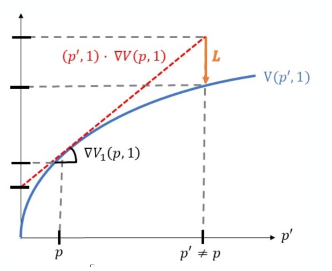
- LPs deposit asset & cash when the asset price is \(p\)
- While in the pool: balanced volume \(V\) + order imbalance \(p\to p'\)
- Withdraw at price \(p'\)
Buy and hold
Provided liquidity
in the pool
- \(\Rightarrow\) positional loss relative to a "buy-and-hold" when \(p'\ne p\)
- adverse selection
- Arbitrageurs monitor the pool
- \(\Rightarrow\) LPs deposit/writhdraw at efficient prices!
Modelling provide-and-forget liquidity provision
\[\int_0^\infty(\underbrace{\Delta c(q^*)-q^*Rp )}_{\text{adverse selection loss when the return is \(R\)}}+ \underbrace{F \cdot \Delta c(q^*))}_{\text{fees earned on informed}}~\phi(R)dR + \underbrace{F\cdot p\cdot V}_{\text{fees earned on balanced flow}}\ge \text{cost of capital}.\]
\(q^* \)= function of \(R\) = what (informed) arbitrageurs trade (net) to move the price to reflect \(R=p'/p\)
Basic idea: LP must earn more fees on balanced flow (in AMM: fees) than what they lose on price movement:
\[\underbrace{\text{what LP sold it for}-\text{value of net position}}_{\text{adverse selection loss}} +\text{fee income} \ge \text{cost of capital} \]
Similar to Lehar and Parlour (2023), Barbon & Ranaldo (2022).
takes the role of the TradFi bid-ask spread
Expected returns to liquidity providers over the "deposit period"
- \(R\) = asset return
- \(F\) = trading fee
- \(V\) = balanced volume
- \(a\) = size of the liquidity pool
Similar to Lehar and Parlour (2023), Barbon & Ranaldo (2022).
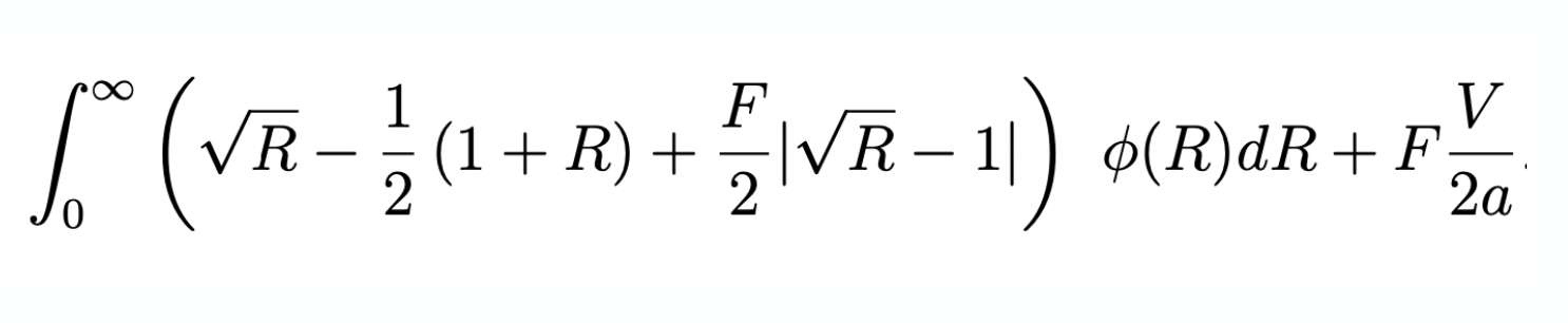
(incremental) adverse selection loss \(L\) when the asset return is \(R=p'/p\)
fees earned
on informed
fees earned
on balanced flow
for reference:
- If the asset price \(\searrow\) 10% the incremental loss \(L\) for liquidity providers is 13 basis points on the deposit
- \(\to\) total loss=-10.13%
- If the asset price \(\nearrow\) 10%, the liquidity provider gains 12 basis points less on the deposit
- \(\to\) total gain =9.88%
For fixed balanced volume \(V\) & fee \(F\):
- Larger pool size \(a \to\) smaller shares of the fees
- \(\Rightarrow \) LP return \(\searrow\) in pool size
-
Competitive liquidty provision:
- \(\Rightarrow\) the upper-bound on pool size above which LPs lose money
- we characterize this by \(\bar{\alpha}\) \(=\) fraction of the asset's market cap to be deposited to the pool
\(=\) 0
Liquidity Demander's Decision & (optimal) AMM Fees
- This calibration: better off with AMM relative to traditional market if
\[\text{AMM price impact} +\text{AMM fee } F \le \text{bid-ask spread}.\]
- Two opposing forces when fee \(F\nearrow\)
- more liquidity provision
\(\to\) lower price impact - more fees to pay
- more liquidity provision
Result:
competitive liq provision\(\to\) there exists an optimal (min trading costs) fee \(F >0\)
- \(\to\) derive closed form solution
- Fee \(F\) depends on asset return distribution, balanced volume, quantity demanded
Similar to Lehar&Parlour (2023) and Hasbrouck, Riviera, Saleh (2023)
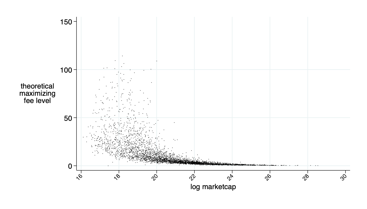
- Optimal \(F\) is asset-specific to compensate LPs for asset-specific adverse selection losses!
- Assumption: asset returns are exogenous to trading (efficient prices)
\[F=\frac{1}{E[|\sqrt{R}-1|/2]+E[V]}\left(-2q\ E[\text{position loss L}]+ \sqrt{-2qV\ E[\text{position loss L}]}\right).\]
Sidebar: modelling adverse selection in traditional microstructure vs. AMM
Traditional microstructure models:
- tick-by-tick analysis
- market makers earn bid-ask spreads
- able to liquidate positions at (favourable to them) inefficient prices
- key modelling variable: informed vs. uninformed order flow (PIN)
AMM (provide-and-forget version):
- liquidity providers are passive, long(er) term (daily horizons)
- liquidity deposits and withdrawals occur at efficient prices
- no positional gains
- key modelling variables
- end-of-day prices (assumed efficient) \(\to\) open-to-close returns
- balanced volume
What's next?
- Calibrate to stock markets
- AMM Feasible?
- Are the AMM costs at the optimal fee \(F\) \(<\) bid-ask spread?
Approach: daily AMM deposits
- AMMs close overnight.
- Market: opening auction \(\to\) initial price \(p\)
- Determine optimal fee \(F\);
LPs deposit \(a\) assets and \(c\) cash at ratio \(p=c/a\) until break even \(\alpha=\overline{\alpha}\)
- Liquidity locked for the day
- At EOD release deposits and fees
- Back to 1.
Background on Data
Special Consideration 1: What volume?
-
some volume may be intermediated
- with AMMs: no need for intermediation
- \(\to\) intermediated volume could disappear
- \(\to\) use volume/2
- Some caveats, e.g.
- arbitrageur volumes
- larger volume if AMM has lower trading costs
Special Consideration 2: What's \(q\) (the representative order size)?
- use average per day
- take long-run average + 2 std of daily averages
- (also avg \(\times 2\),\(\times 4\), depth)
All displayed data CRSP \(\cap\) WRDS
- CRSP for shares outstanding
- WRDS-computed statistics for
- quoted spreads (results similar for effective)
- volume
- open-to-close returns
- average trade sizes, VWAP
- Time horizon: 2014 - March 2022
- Exclude "tick pilot" period (Oct 2016-Oct 2018)
- All common stocks (not ETFs) (~7550).
- Explicitly not cutting by price or size
- All "boundless" numbers are winsorized at 99%.
Special Consideration 3:
Where to get returns and volume?
- Approach 1: "ad hoc"
- "one-day-back" look
- take yesterday's return and volume when deciding on liquidity provision in AMM
- Approach 2: estimate historical return distribution
(Most of) the slides coming up: AMMs based on historical returns
- average \(F^\pi=11\)bps
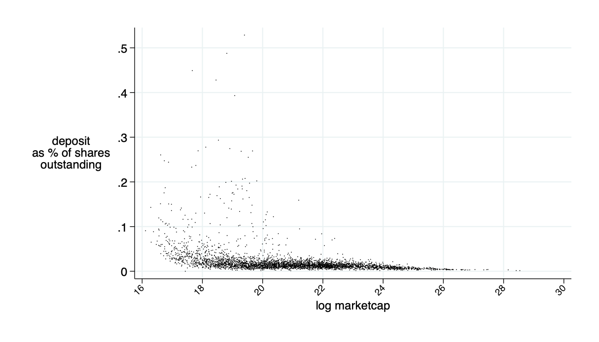
Average of the market cap to be deposited for competitive liquidity provision: \(\bar{\alpha}\approx 2\%\)
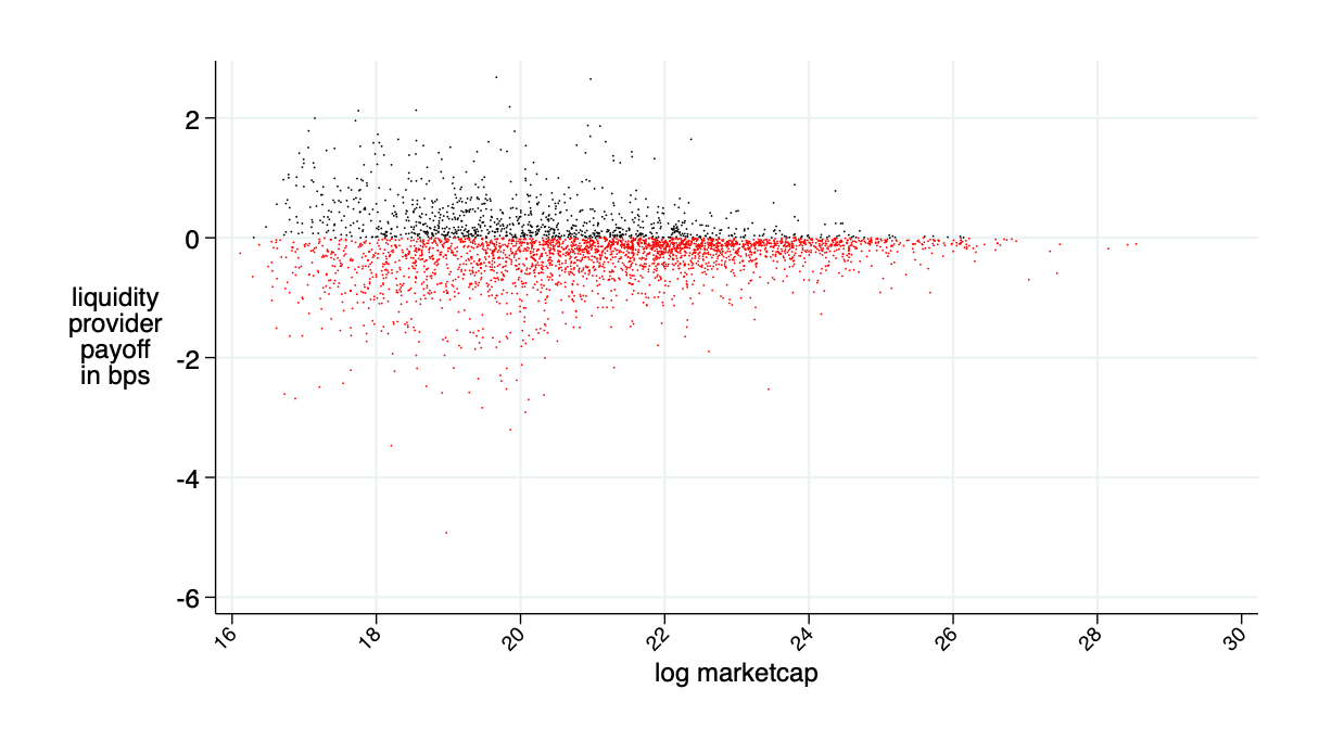
almost break even on average (average loss 0.2bps \(\approx0\))
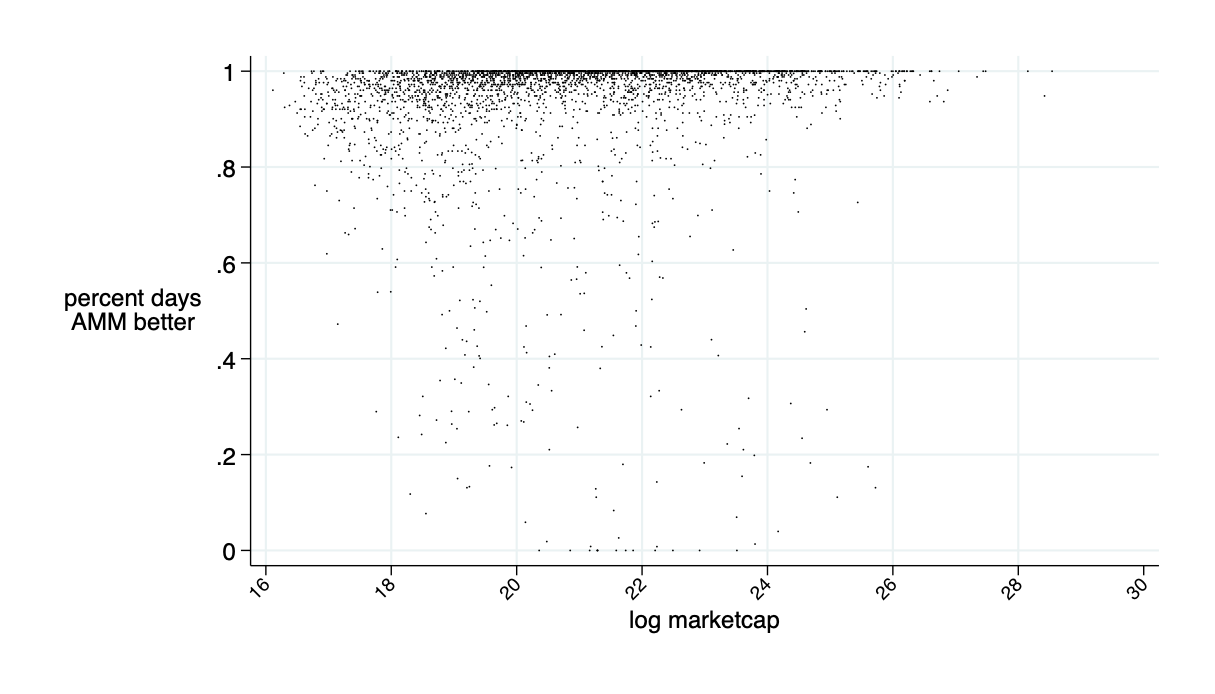
average: 94% of days AMM is cheaper than LOB for liq demanders
AMMs are better on about 85% of trading days
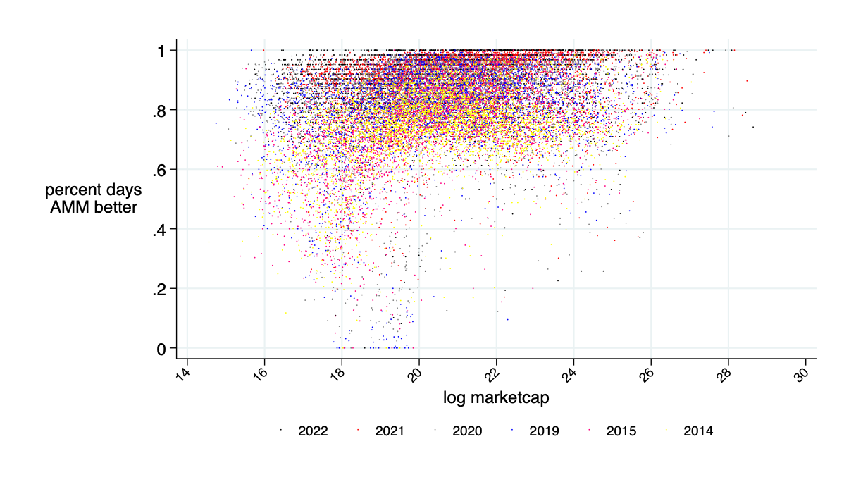
AMMs with"ad hoc" one-day backward look
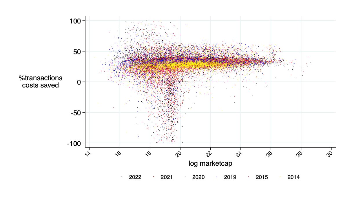
relative savings: what fraction of transactions costs would an AMM save? \(\to\) about 30%
AMMs with"ad hoc" one-day backward look
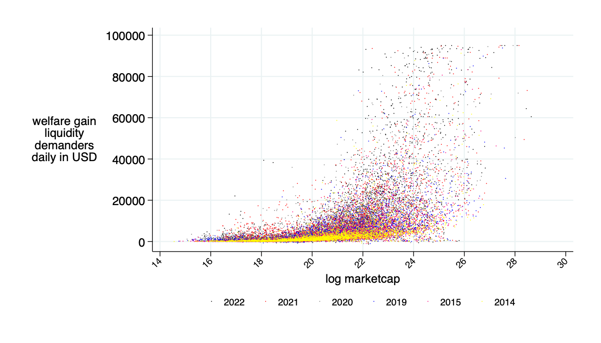
average per-day savings: 16 bps
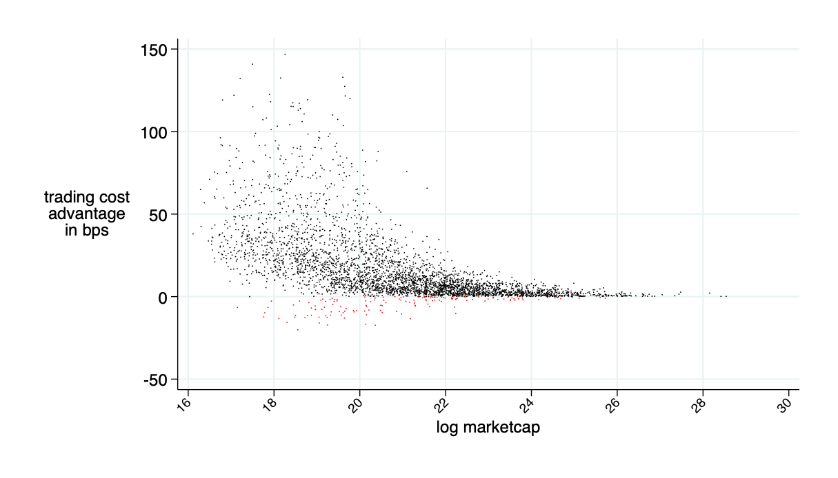
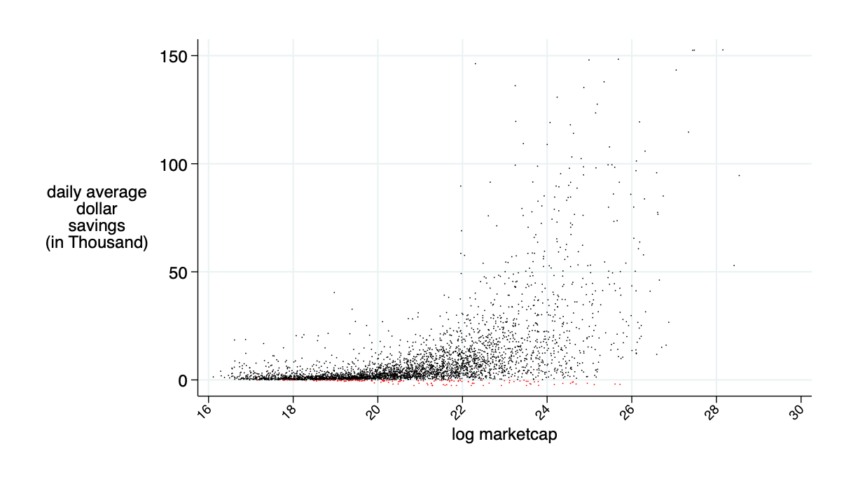
average daily: $9.5K
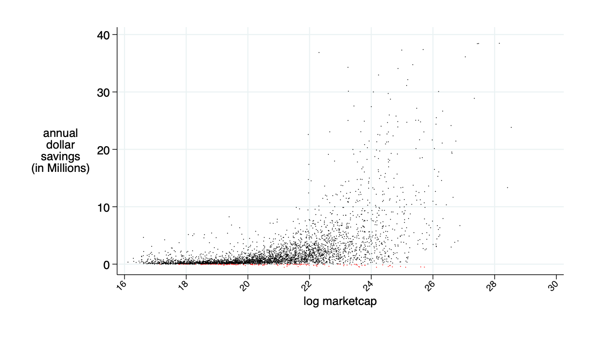
average annual saving: $2.4 million
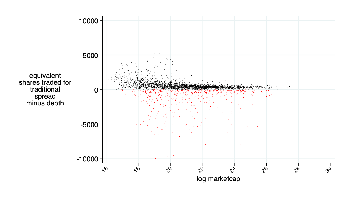
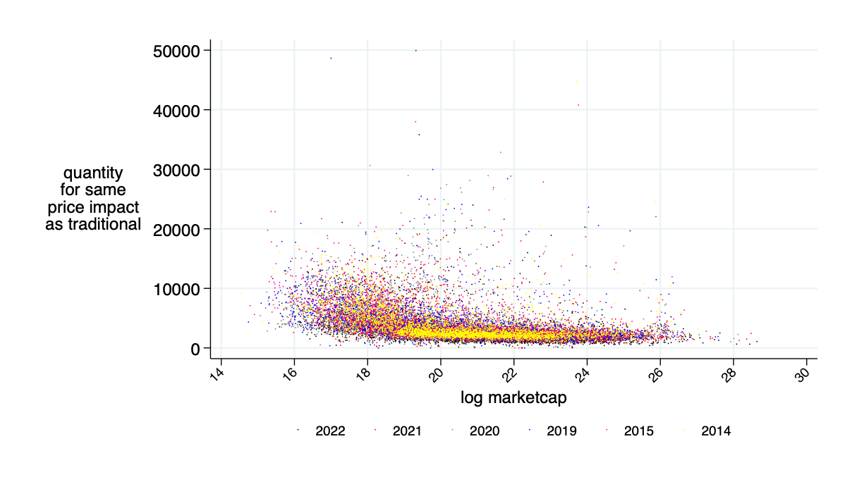
implied "excess depth" on AMM relative to the traditional market
Sidebar 1: constant product AMM vs Traditional Pricing Models
AMM constant product pricing is the same as a LOB under minimal assumptions:
- prices are continuous
- the marginal price are determined by the ratio of the liquidity deposits in the pool
Basic Requirements for "unconstrained" two-asset liquidity pool
- Two assets:
- cash and an asset
- deposits in pool of \(c\) cash and \(a\) asset
- AMMs should be self-contained: pricing rule based on
- deposits \(a,c\) and
- liquidity demanded \(q\)
- implied value of the asset at deposit: \[p=\frac{c}{a}.\]
- \(\to\) marginal price: an infinitesimal unit should cost \[p^m=p\]
What does an AMM need?
- What happens with trades?
- a trade of \(q\in(-\infty,a),\) will cost \(\Delta c(q)\)
- liquidity changes
- \(a\) \(\to\) \(a-q\)
- \(c\) \(\to\) \(c+\Delta c(q)\)
- \(\to\) marginal price after trade of \(q\) is
\[p^m(0)=\frac{c}{a}~~\to~~p^m(q)=\frac{c+\Delta c(q)}{a-q}.\]
What is this cost in traditional pricing models?
Pricing Rules from Traditional Markets: Uniform Price
- cost is price \(\times\) quantity: \[\Delta c(q)=q\cdot p^m(q)\]
- plus assume average price \(=\) marginal price after trade
\[p^m(q)=\frac{c+q\cdot p^m(q)}{a-q}~~\Leftrightarrow~~p^m(q)=\frac{c}{a-2q}.\]
- formalized and analyzed by Canidio and Fritsch (2023) and implemented in COW-Swap
- execute all trades at a marginal price after a batch
- \(\to\) no positional loss for LPs
- Concern: order splitting by liquidity demanders
- Is the Electronic Limit Order Book Inevitable (Glosten 1994)
Pricing Rules from Traditional Markets: Limit Order Book
- Liquidity providers submit sell orders \(s_1(p_1,q_1),\ldots,s(p_n,q_n)\)
- Matching engine sorts order increasing by price
-
someone who wants to buy quantity \(q\)
\[\Delta c(q)=\sum_{i=1}^mq_i\cdot p_i.\]
- Assume the price-quantity curve can be expressed by a continuous marginal price function \(p^m(s) \)
\[\to \Delta c(q)=\int_0^qp^m(s) ds.\]
note: if you do uniform pricing and split your order into infinitesimal units, then you pay the limit order price
LOB-style pricing in AMM \(\to\) constant product pricing
- Continuity \(\to\) price of "final" marginal unit coincides with price of "first" marginal unit of next trade \[\Delta c(q)=\int_0^q p^m(s) ds~\to~\Delta c'(q)=p^m(q).\]
- \(\to\) a differential equation
- \[p^m(q)=\frac{c+\Delta c(q) }{a-q}~~\Leftrightarrow~~\Delta c'(q)=\frac{c+\Delta c(q)}{a-q},\]
- Also "first" unit costs nothing \(\Delta c(0)=0\)
- \(\to\) solution \[\Delta c(q)=q\cdot\frac{c}{a-q}.\]
AMM constant product pricing is the same as a LOB under minimal assumptions:
- prices are continuous
- the marginal price are determined by the ratio of the liquidity deposits in the pool
Most Common Pricing Rule in DeFi: Constant Product
- For AMM: assume "constant" liquidity
- Liquidity defined as product of deposits
-
\(\to\) liquidity before and after trade coincides
\[a\cdot c= (a-q) (c+\Delta c(q))\] -
This implies cost
\[\Delta c(q)=q \frac{c}{a-q},\] average price \[p(q)=\frac{c}{a-q}\]
and marginal price \[p^m(q)=\frac{c+\frac{cq}{a-q}}{a-q}=\frac{ac}{(a-q)^2}.\]
Insight: AMM pricing function is the same as a limit order book when we require
- that prices are continuous and
- that prices are determined by liquidity deposits only
Sidebar 2: Cash deposit requirements
- Asset provision is not a problem: enough idle liquidity
-
But: AMM requires off-setting cash: \(c =a\cdot p\).
- Cash is not free: at 4.5% annual rate, 1.75bps per day.
- Adds to fees
- Several solutions:
- Narrow a range of returns for which to provide liquidity (akin to Uniswap V3) or circuit breakers
- Other mechanisms being developed
- Use the same cash for many assets (Balancer protocol)
\(\Rightarrow \) Need about 5% of the value of the shares deposited -- not 100% -- to cover up to a 10% return decline
Sidebar 1: Deposit Requirements/Uniswap V3
- Our approach: measure liquidity provision in % of market cap
- Share-based liquidity provision is not a big issue: the shares are just sitting at brokerages.
- But: AMM requires an off-setting cash amount: \(c =a\cdot p\).
- Cash is not free:
- at 4.5% annual rate, must pay 1.75bps per day.
- Would need to add to fees
- But: do we need "all that cash"?
- No.
- (hand-waving argument)
- 2nd gen AMMs have liquidity provision "bands": specify price range for which one supplies liquidity
-
Equity markets: have curcuit breakers
- \(\to\) specify range for \(R\in(\underline{R},\overline{R})\)
- Outside range: don't trade
- Inside range: "full" liquidity with constant product
formula.
- Implication: only need cash and shares to satisfy
in-range liquidity demand.
\(\Rightarrow \) Need about 5% of the value of the shares deposited -- not 100% -- to cover up to a 10% return decline
Other solutions in the works: e.g., Balancer Protocol
Sidebar 1: Deposit Requirements/Uniswap V3
- Uniswap V3 allow LPs to provide liquidity only when price is in interval \([\underline{p},\overline{p}]\)
- \(\to\) conceptually similar to circuit breakers
-
Hasbrouck, Riviera, Saleh ( 2025): concerntrated liquidity provision \(\to\) payoff same as a covered call.
- liquidity provision decision requires constant adjustments,
- indirectly related to the concept of LVR=loss-vs-rebalancing)
- modelling caveat: because price interval is a choice, too many degrees of freedom
Summary
- AMMs do not require a blockchain - just a concept
- could be run in the existing world (though there are institutional and regulatory barriers)
- Our question:
- Can an economically viable AMM be designed for current equity markets?
- Would such an AMM improve current markets?
- Answers:
- Yes.
- Massively.
- Source of Savings:
- Liquidity providers \(\not=\) Citadel!
- \(\to\) no (overnight) inventory costs
- \(\to\) use idle capital
- \(\to\) + better risk sharing
Summary: alternative view
- AMMs force LPs to optimize against a prescribed, fully contingent limit order book function
- the positional loss and the break-even condition that we derive does not require strong assumptions such as behavior or number of informed traders
- a positonal loss for LPs will occur
-
LPs will receive compensation through fees
- based on calibration data, LPs would break even with this specification
- \(\to\) a form of lower bar for trading costs? Compensating for adv selection only
- \(\to\) that lower bar is not reached maybe tells us something about the competitiveness/frictions in the present market?

@katyamalinova

malinovk@mcmaster.ca

slides.com/kmalinova

https://sites.google.com/site/katyamalinova/
Basic Requirements for "unconstrained" two-asset liquidity pool
- Two assets:
- cash and an asset
- deposits in pool of \(c\) cash and \(a\) asset
- AMMs should be self-contained: pricing rule based on
- deposits \(a,c\) and
- liquidity demanded \(q\)
- implied value of the asset at deposit: \[p=\frac{c}{a}.\]
- marginal price: an infinitesimal unit should cost \[p^m=p\]
What does an AMM need?
- trades create linear changes:
- a trade of \(q\in(-\infty,a),\) will cost \(\Delta c(q)\)
- liquidity changes
- \(a\) \(\to\) \(a-q\)
- \(c\) \(\to\) \(c+\Delta c(q)\)
- \(\to\) marginal price after trade of \(q\) is
\[p^m(0)=\frac{c}{a}~~\to~~p^m(q)=\frac{c+\Delta c(q)}{a-q}.\]
Some Pricing Rules from Traditional Markets: Uniform Price
- assume cost is price \(\times\) quantity: \[\Delta c(q)=q\cdot p^m(q)\]
- plus assume average price \(=\) marginal price after trade
\[p^m(q)=\frac{c+q\cdot p^m(q)}{a-q}~~\Leftrightarrow~~p^m(q)=\frac{c}{a-2q}.\]
- formalized and analyzed by Canidio and Fritsch (2023) and implemented in COW-Swap
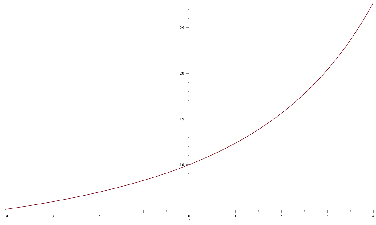
\(q=2\)
Example: \(\Delta c(q)= q\times p^m(q)=2\times 15.5\)
Main pricing rule in stock exchanges: limit order book

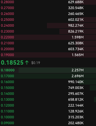
quantity
price
\(q\)
\(p^m(q)\)
\(\Delta c(q)=\int_0^qp^m(s)~ds\)
again note: the marginal pricing function \(p(q)\) does not have to be linear
Some Pricing Rules from Traditional Markets: Limit Order Book
- For AMM: assume continuity \(\to\) price of "final" marginal unit coincides with price of "first" marginal unit of next trade \[\Delta c(q)=\int_0^q p^m(s) ds~\to~\Delta c'(q)=p^m(q).\]
- Also "first" unit costs nothing \(\Delta c(0)=0\)
- This gives us a differential equation
\[p^m(q)=\frac{c+\Delta c(q) }{a-q}~~\Leftrightarrow~~\Delta c'(q)=\frac{c+\Delta c(q)}{a-q},\] - with solution \[\Delta c(q)=q\cdot\frac{c}{a-q}.\]
Most Common Pricing Rule in DeFi: Constant Product
- With \[a\cdot c= (a-q) (c+\Delta c(q))\]
-
we compute cost \[\Delta c(q)=q\cdot \frac{c}{a-q},\]
- and marginal price \[p^m(q)=\frac{c+\frac{cq}{a-q}}{a-q}=\frac{ac}{(a-q)^2}.\]
Insight: AMM pricing function is the same as a limit order book when we require
- that prices are continuous and
- that prices are determined by liquidity deposits only
- price \(\times\) quantity: \[p(q)=\frac{c}{a-2q}\]
- limit order book: \[p(q)=\frac{c}{a-q}.\]
- constant product: \[p(q)=\frac{c}{a-q}.\]
average prices
Some insights on pricing functions
- Price \(\times\) quantity
- nice feature:
- regret-free price: if price move is due to information, you have no positional loss
- poor feature:
- you can always save by order-splitting (formally shown by Canidio and Fritsch (2023))
- limit price for splitting = limit order book price
- nice feature:
- LOB/CP
- nice feature:
- order splitting doesn't pay
- poor feature:
- prices not regret-free: if price move is due to information, you always lose
- nice feature:
Optimally Designed AMMs with
"ad hoc" one-day backward look
Optimal fee \(F^\pi\)
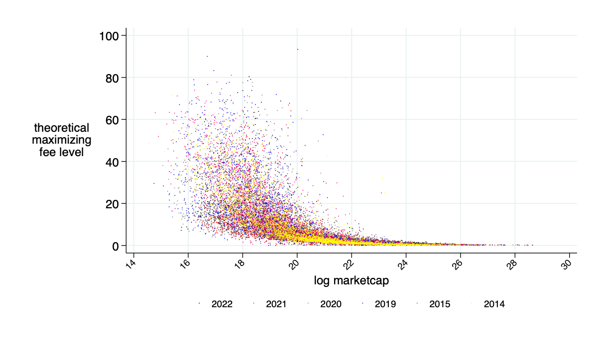
\(\overline{\alpha}\) for \(F=F^\pi\)
Need about 10% of market cap in liquidity deposits to make this work
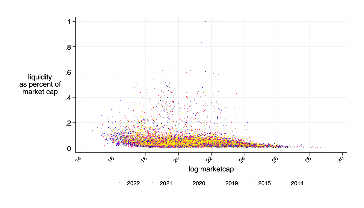
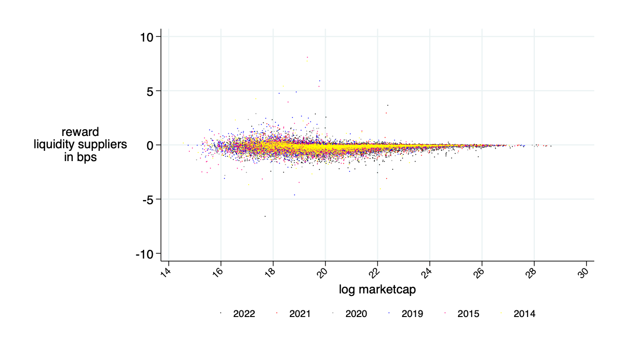
average benefits liquidity provider in bps (average=0)
Insight: Theory is OK - LP's about break even
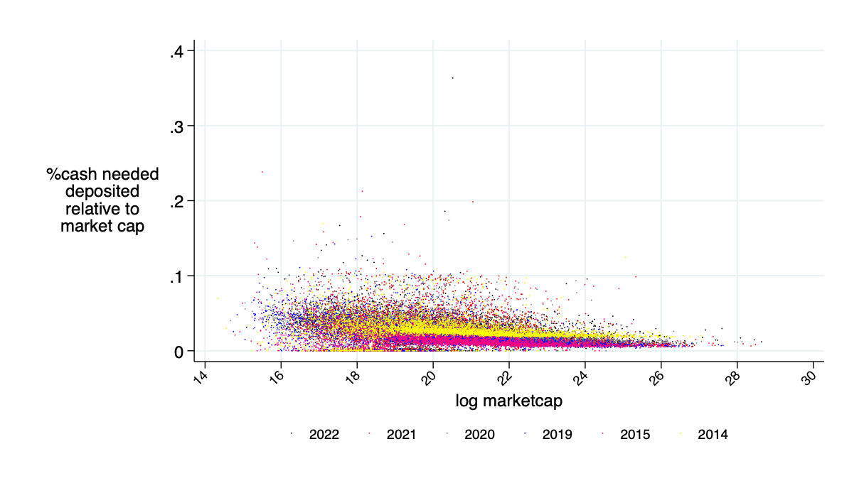
with circuit breakers: what fraction of \(\alpha\) needs to be deposited as cash
Only need about 5% of the 10% marketcap amount in cash
quoted spread minus AMM price impact minus AMM fee (all measured in bps)
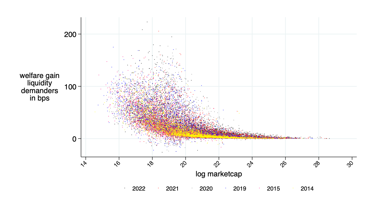
theoretical annual savings in transactions costs is about $15B
Optimal fee \(F^\pi\)
average benefits liquidity provider in bps (average=0)
Insight: Theory is OK - LP's about break even
\(\overline{\alpha}\) for \(F=F^\pi\)
Need about 10% of market cap in liquidity deposits to make this work
actually needed cash as fraction of "headline" amount
Only need about 5% of the 10% marketcap amount in cash
AMMs are better on about 85% of trading days
quoted spread minus AMM price impact minus AMM fee (all measured in bps)
relative savings: what fraction of transactions costs would an AMM save? \(\to\) about 30%
theoretical annual savings in transactions costs is about $15B