Velocity fields and streamlines in 2D
(MMG640 / MVE080)
Overview
- Review: dynamical systems, vector fields, phase portraits
- Velocity field plots in 2D using 'quiver' function
- Task: pendulum quiver plot
- Review: numerical integration algorithms
- Streamline plots in 2D using 'streamline' function
- Task: pendulum streamlines
Dynamical systems
\begin{aligned}
x' &= f(x,y) \\
y' &= g(x,y)
\end{aligned}
X' = F(X)
X=[x,y], F = [f,g]
velocity field

Quiver plot
\displaystyle
\begin{aligned}
x' &= v \\
v' &= -\frac{g}{l}\sin x
\end{aligned}
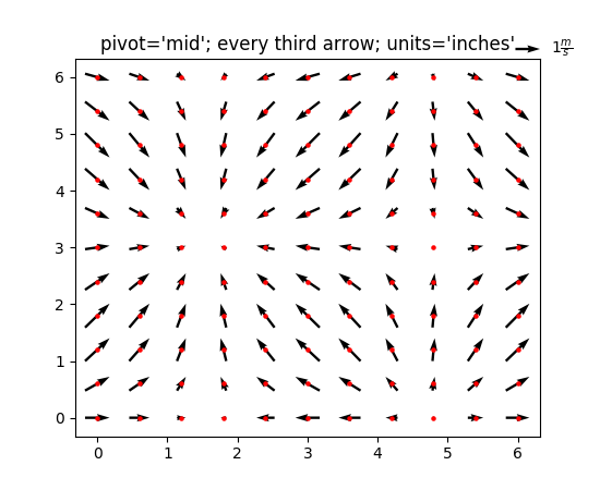
The function 'quiver' in Matplotlib is used for plotting 2D velocity fields
Motion of a pendulum
(Task in Work-sheet 3)
g=10, \quad l=0.1
Phase portrait
\begin{aligned}
x' &= f(x,y) \\
y' &= g(x,y)
\end{aligned}

Integral curves
Streamline plot
Numerical integration
\begin{aligned}
x' &= f(x,y) \\
y' &= g(x,y)
\end{aligned}

Integral curves
Simplest numerical algorithm: Euler's method
\begin{aligned}
x_{k+1} &= x_k + h f(x_k,y_k) \\
y_{k+1} &= y_k + h g(x_k,y_k)
\end{aligned}
Higher-order methods:
Runge-Kutta, etc