Random matrices
and
Quantum Chaos
Outline
- Wigner and random matrices
- Some tricks for building matrices
- Quantum chaos
Short appetizers: with relevant refernces
T. Guhr, A. Mueller-Groeling, H. A. Weidenmueller,Phys.Rept. 299, 189 (1998)
Alan Edelman and Yuyang Wang,"Random Matrix Theory and its Innovative Applications"
and as always Wikipedia and Google are your friends!
Task I
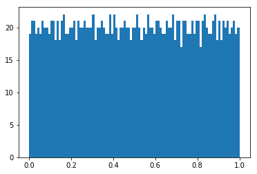
- Diagonal random matrix
a) Generate a 2000x2000 diagonal matrix with uniformly distributed random entries. The mean of the entries should be 0!
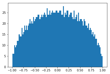
b) Calculate distribution of the eigenvalues.
(i.e. use diag() and rand() and generate a histogram)
- Symmetric full random matrix
a) Generate a 2000x2000 random symmetric matrix who's entries are drawn from the same distribution as above.
b) Calculate distribution of the eigenvalues.
- Try to fit the obtained distributions !
- If bored try other random number generators!
Cheet sheet for fitting
from scipy.optimize import curve_fit # use this for fitting

x # this is a 1D array containing sampling points of the data
y # this is a 1D array containing the data at the sampling points

# We define a function to be used for fitting
# in ths case we fit a sin
def fun(x,A,w,phi):                # The signature is important!
                                   # First argument corresponds to sampling!
    return A*sin(w*x+phi)          # This is just a simple sine
                                   # with the usual  parameters

#fitting is done like this
popt,pcov=curve_fit(fun,x,y)

popt               # parameters of the fit go here
sqrt(diag(pcov))   # errors of the parameters are
                   # obtained from the covariance matrix


fun(x,*popt) # this will evaluate the fitted function at the sampling points
Wigner's semicircle
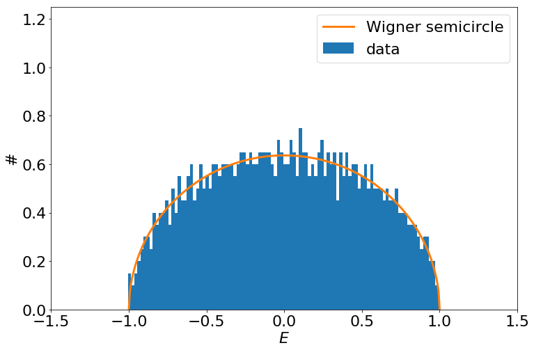
Wigner's semicircle
- Wigner's approach for tackling spectra of large nuclei.
(Annals of Mathematics, 62 548, 1955)
- Large truly random matrices tend to have a semicircular eigenvalue distribution.
"Central limit theorem for matrices"
- Wigner's original proof concerned normally distributed matrix elements and thus he was able to match moments of the eigenvalue distribution to a semicircle.
Road to universality: Unfolding spectra
unfolded sample
having uniform distribution
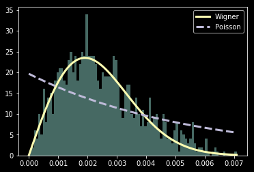
Wigner's surmise: level spacings are universal
Wigner conjectured that the distribution of the unfolded level spacings shows universal behavior...
universality class
normalization
Integrable systems
Generic 'chaotic' systems
correlated levels
"repel" eachother
"uncorrelated" levels
can be arbitrarily close
Gaussian ensembles
-
Gaussian orthogonal ensemble (GOE),β=1
Systems with time reversal symmetry
Symmetric matrices, normally distributed real elements
-
Gaussian unitary ensemble (GUE),β=2
Generic systems without any symmetry
Hermitian matrices, normally distributed complex elements
- Gaussian symplectic ensemble (GSE),β=4
Systems with spin rotational symmetry
Symmetric matrices, normally distributed real quaternio elements
How to unfold in practice
from scipy import interpolate # we will need interpolate data
ev=eigvalsh(H)                # get some eigenvalues

# generate the cumulative distribution of the eigenvalues
# here we use matplotlib's hist
# could use numpy's but it has no built in cumulative histogram ...
hg=hist(ev,100,cumulative=True,normed=True) # may need to play with bins

# interpolate the cumulative
# careful ! histogram generators give one more bin
ipol=interpolate.interp1d(hg[1][1:],hg[0],
                        fill_value=(0,1),bounds_error=False)
# these last options are needed to treat the edge properly


# unfolded eigenvalues
unfolded_ev=ipol(ev))
Task II
-
Generate a 2000x2000 random diagonal matrix.
- Generate 2000x2000 random matrices from Gaussian orthogonal and unitary ensembles. (If bored generate also a matrix from the symplectic ensamble!)
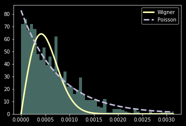
- Calculate distribution of level spacings for each matrix generated. Verify that the unfolded distribution is described by the Wigner surmise or Poisson law!
Matrix building tricks
Goal: Solve the Schrödinger equation for biliard systems
Laplacian on a lattice
2D Hamiltonians
y
x
Hard wall potential is realized by omitting well chosen points from the grid!
But how do I build these matrices?
diag(ones(3))
>>array([[1., 0., 0.],
         [0., 1., 0.],
         [0., 0., 1.]])
diag(ones(2),1)
>>array([[0., 1., 0.],
         [0., 0., 1.],
         [0., 0., 0.]])
kron(array([[1,0,0],
[0,1,0],
[0,0,1]]),
array([[1,2],
[3,4]])
)
>>array([[1., 2., 0., 0., 0., 0.],
[3., 4., 0., 0., 0., 0.],
[0., 0., 1., 2., 0., 0.],
[0., 0., 3., 4., 0., 0.],
[0., 0., 0., 0., 1., 2.],
[0., 0., 0., 0., 3., 4.]])Matrices with entries on
diagonals can be built with
diag()
Use kron() to build hypermatrices
Use numpy array slicing for defining the shape !!
x,y=meshgrid(...) # when defineing the lattice
                  # keep the coordinates close at hand!!

x=x.flatten()     # flatten meshgrid generated matrices
y=y.flatten()     # so we can use coordinates for indexing
...
H # let this be a Hamiltonian
  # of a regular lattice

H_potato=H[:,f(x,y)<0][f(x,y)<0,:] # bool expressions
                                   # can be used for slicing
Solving the eigensystem
va=eigenvals(H)   # only eigenvalues

va,ve=eigh(H)     # eigenvalues AND eigenvectors

# if using numpy arrays @ is the dot product
# if using numpy matrices * is the dot product
H@ve[:,i]=va[i]*ve[:,i] # the i-th eigenvector and eigenvalue satisfy this

# if coordinates of the tracked degrees of freedom
# are stored in the variables x,y

tripcolor(x,y,abs(ve[:,i])**2) # this will visualize the i-th eigenvector
Sparse matrices
# these are modules to deal with sparse matrices
import scipy.sparse as ss
import scipy.sparse.linalg as sl

# matrix building functions have sparse alternatives
idL=ss.eye(L)                    # identity
odL=ss.diags(ones(L-1),1,(L,L))  # off diagonal

ss.kron(A,B) # kron is also here

# cut region of interest
Hsliced=H[:,slice][slice,:]            # slicing works if sparse
Hsliced=(H.tocsr())[:,slice][slice,:]  # csr format is used
                                       # casting from other formats
                                       # might be needed

# Some (strictly not all) eigenvalues can be obtained
# Lanczos and Arnoldi algorithms are used in the background
va,ve=sl.eigsh(Hsliced,30,sigma=0.5)   # this gets 30 eigenvalues
                                       # and eigenvectors from around 0.5
Task III
- Generate Hamiltonian of a 2D particle on a lattice in a rectangle region.
- Generate Hamiltonian in an arbitrary potato shaped region.
- Find lowest couple of eigenvalues (eigenvectors as well if bored)
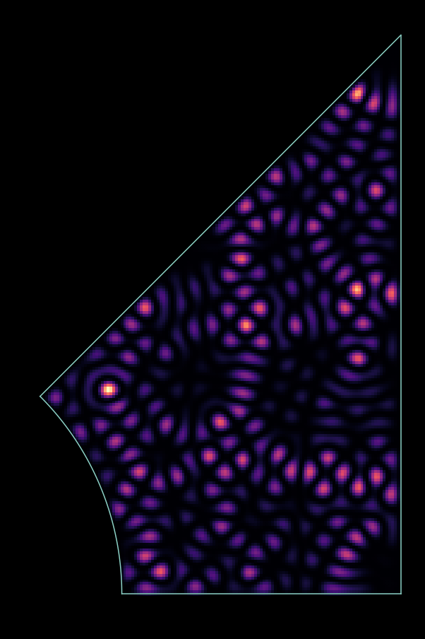
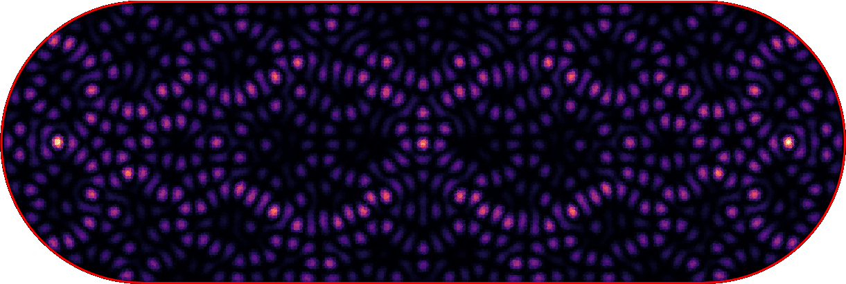
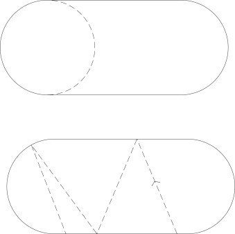
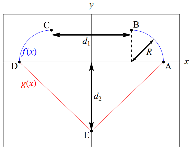
- Investigate the Sinai billiard in the integrable (R=0) and chaotic limit (R>0).
a) Generate a Hamiltonian for the system in the picture.
(give max 4000x4000 matrices to eig() )
b) Calculate unfolded eigenvalues.
c) Calculate level spacing distribution for
both cases.

Extra: explore other billiards
- Elipse
- Bunimovich stadium
- Diamond
- Add magnetic field for GUE biliards

- get rid of all rotational and mirror symmetries
- go for larger grids with sparse matrices
Quantum Chaos -> Wigner surmise
R=0
R=1
Some considerations
- Discretization can make integrable seem chaotic.
(Wigner instead of Poisson) - Spurious symmetries can make chaotic seem integrable. (Poisson instead of Wigner)
- In order to get rid of artifacts grid may need to be large.
- Adaptive grid can help discretization error.
- Sparse matrices and Lanczos algorithm can be used to get reasonable amount of data in reasonably short time.