行動技術與應用
Lesson 8: TensorFlow / Keras with R

迷思:AI新創公司到處都有
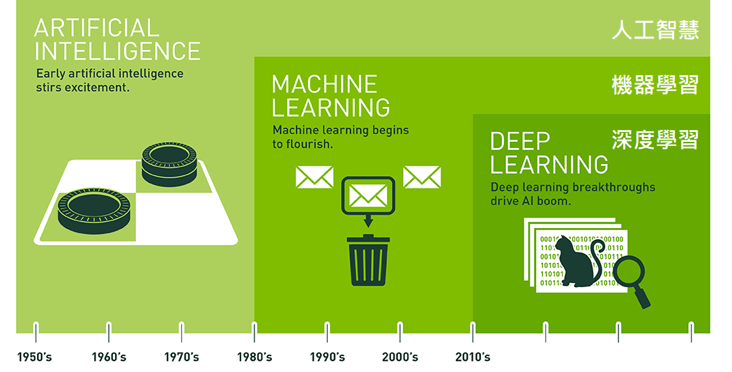
迷思:人工智慧就是深度學習
人工智慧的演進

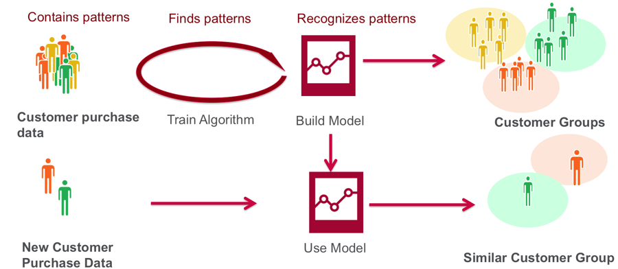
機器學習
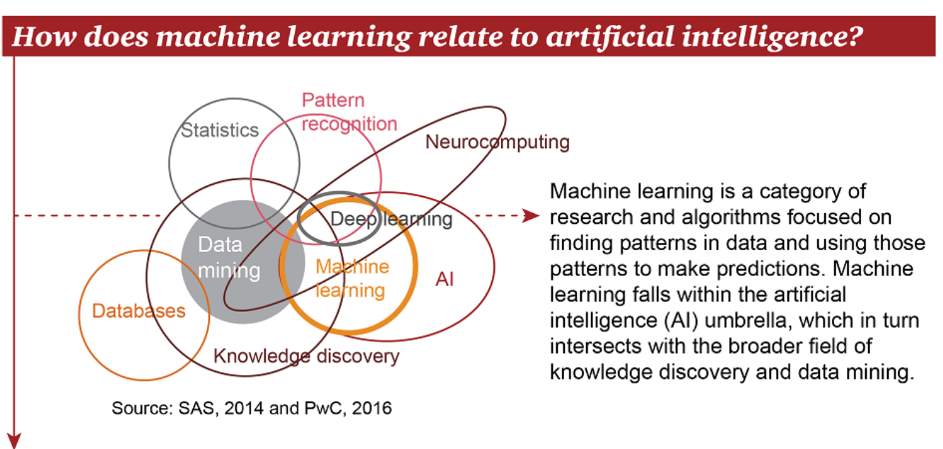
找出patterns
預測未來
訓練集

驗證集
測試集
建立模型
驗證模型
測試模型
使用模型
調校
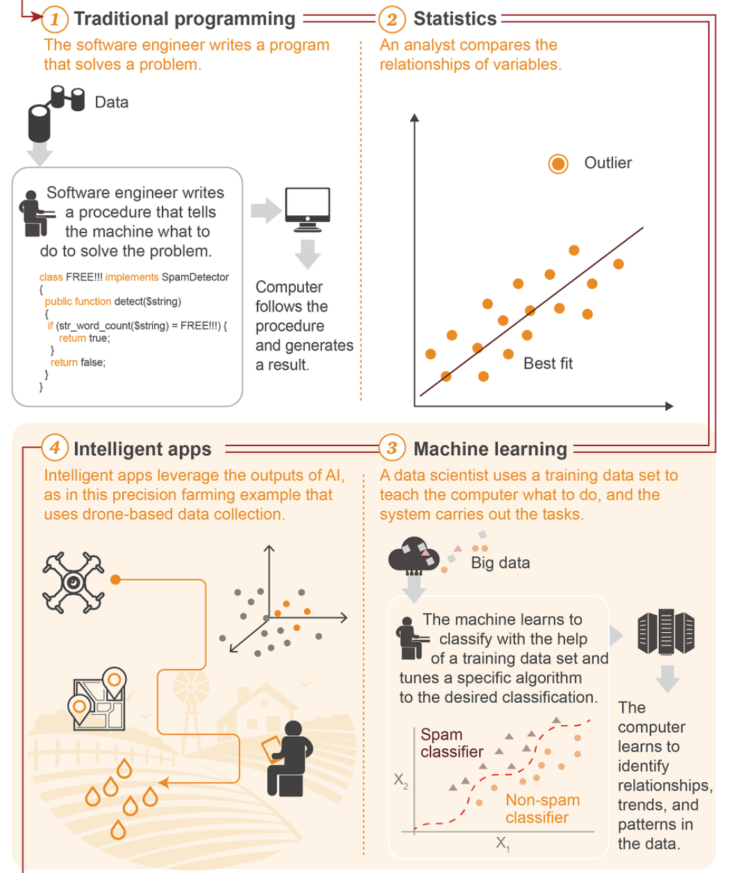
程式設計師
資料分析師
資料科學家
應用
機器學習演算法
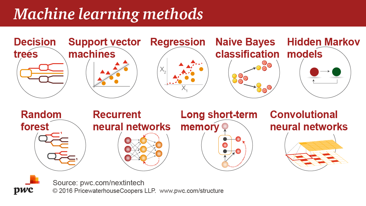
機器學習決策樹
https://usblogs.pwc.com/emerging-technology/wp-content/uploads/2017/04/Machine_Learning_Twitter_2.png
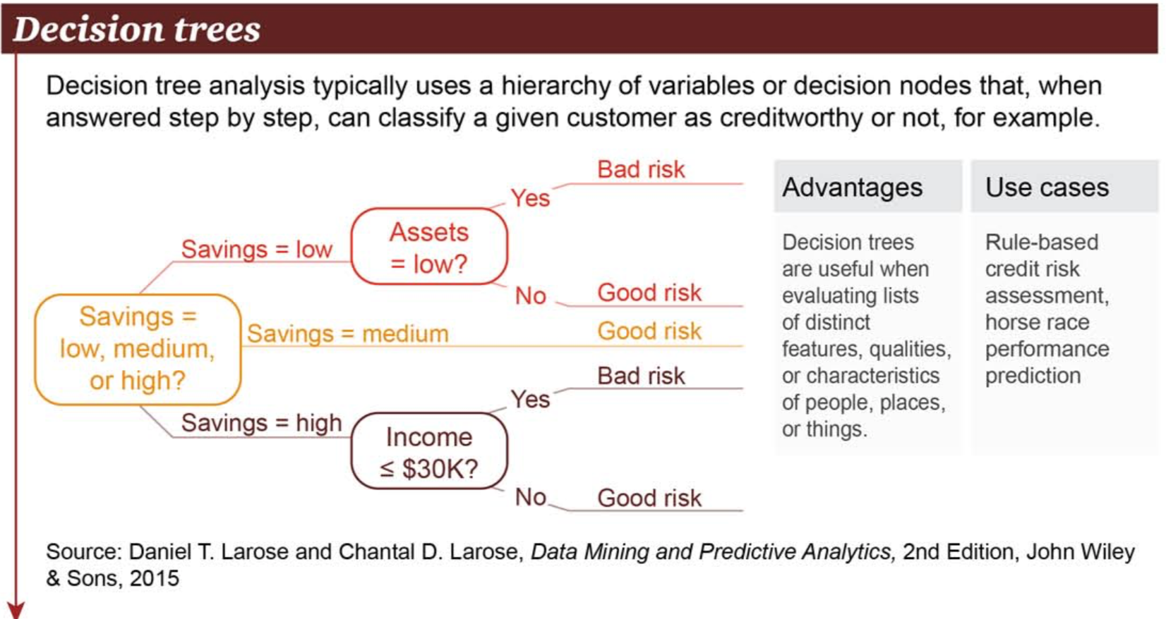
貸款風險評估
儲蓄
動產/不動產
機器學習決策樹
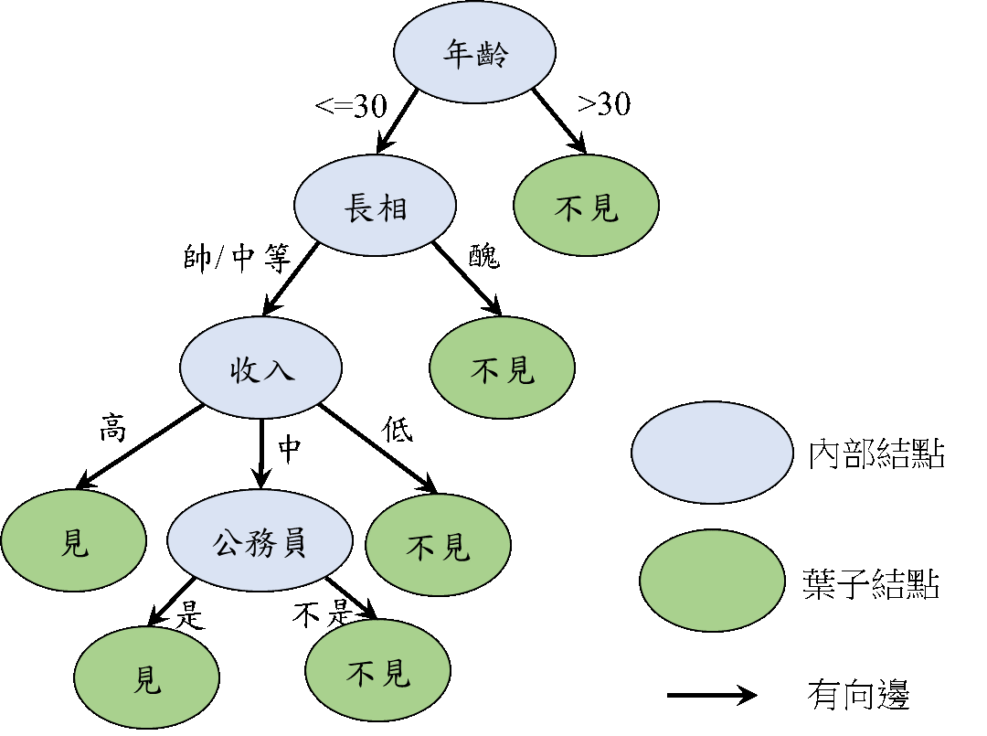
相親決策樹
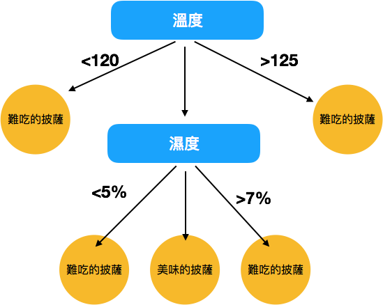
烘烤披薩的過程
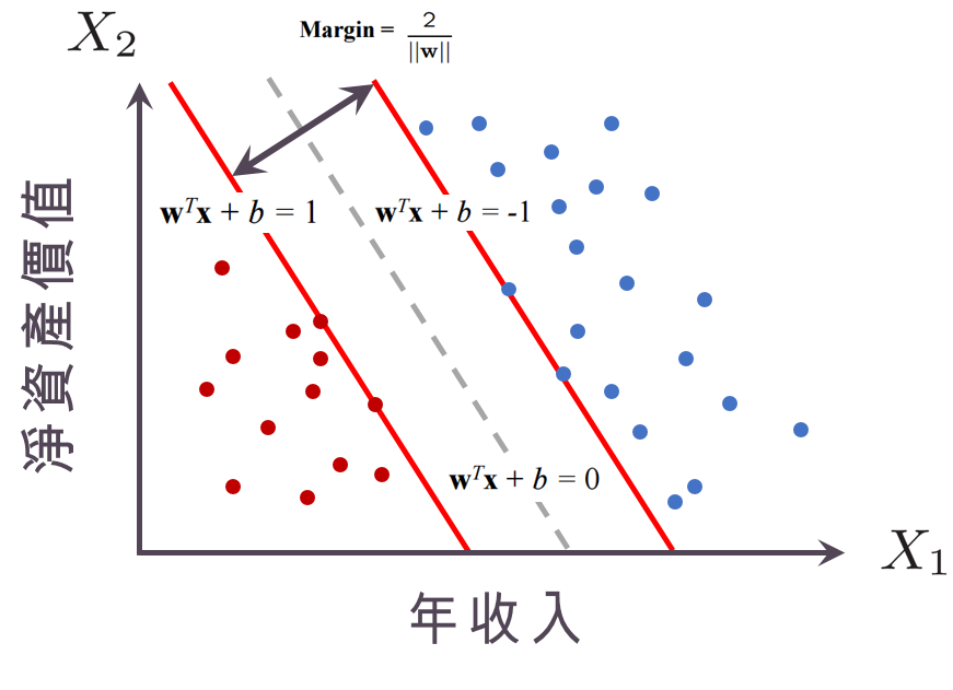
機器學習支持向量機
https://usblogs.pwc.com/emerging-technology/wp-content/uploads/2017/04/Machine_Learning_Twitter_2.png
超平面
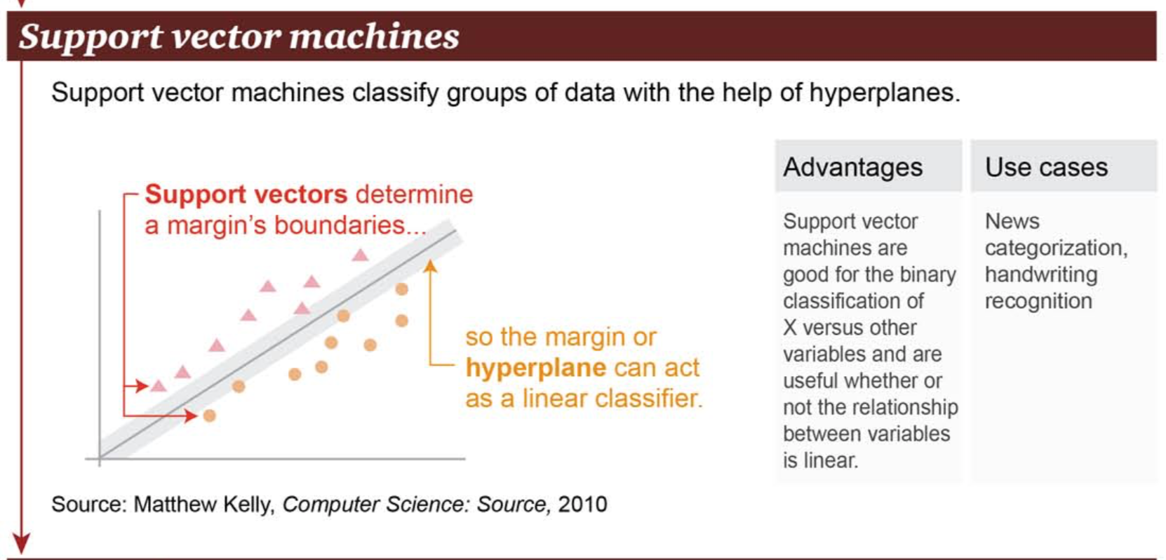
分類問題
機器學習支持向量機
資料來源: 讀者提問:什麼是支持向量機 (SVM)
❸最好的超平面:離兩邊的點都夠遠
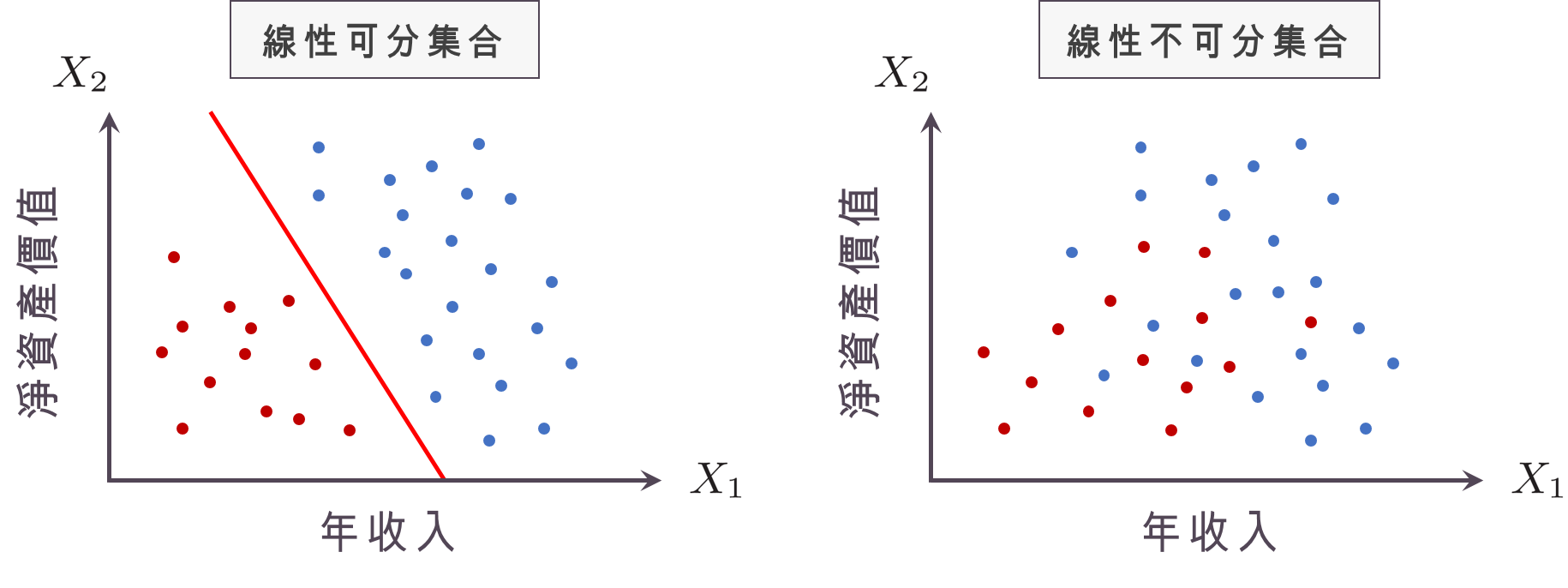
❶資料集必須可分類
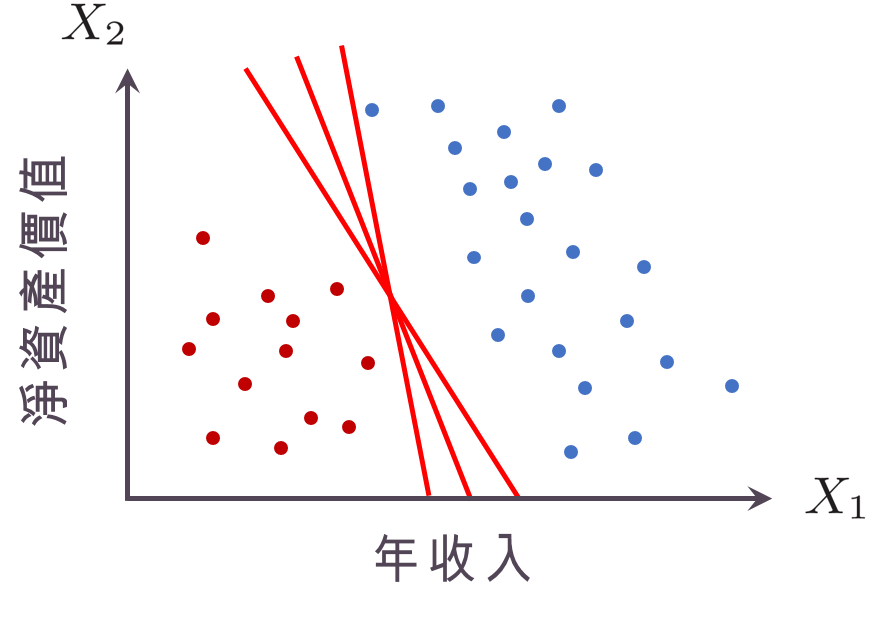
❷哪一個平面分得比較好?
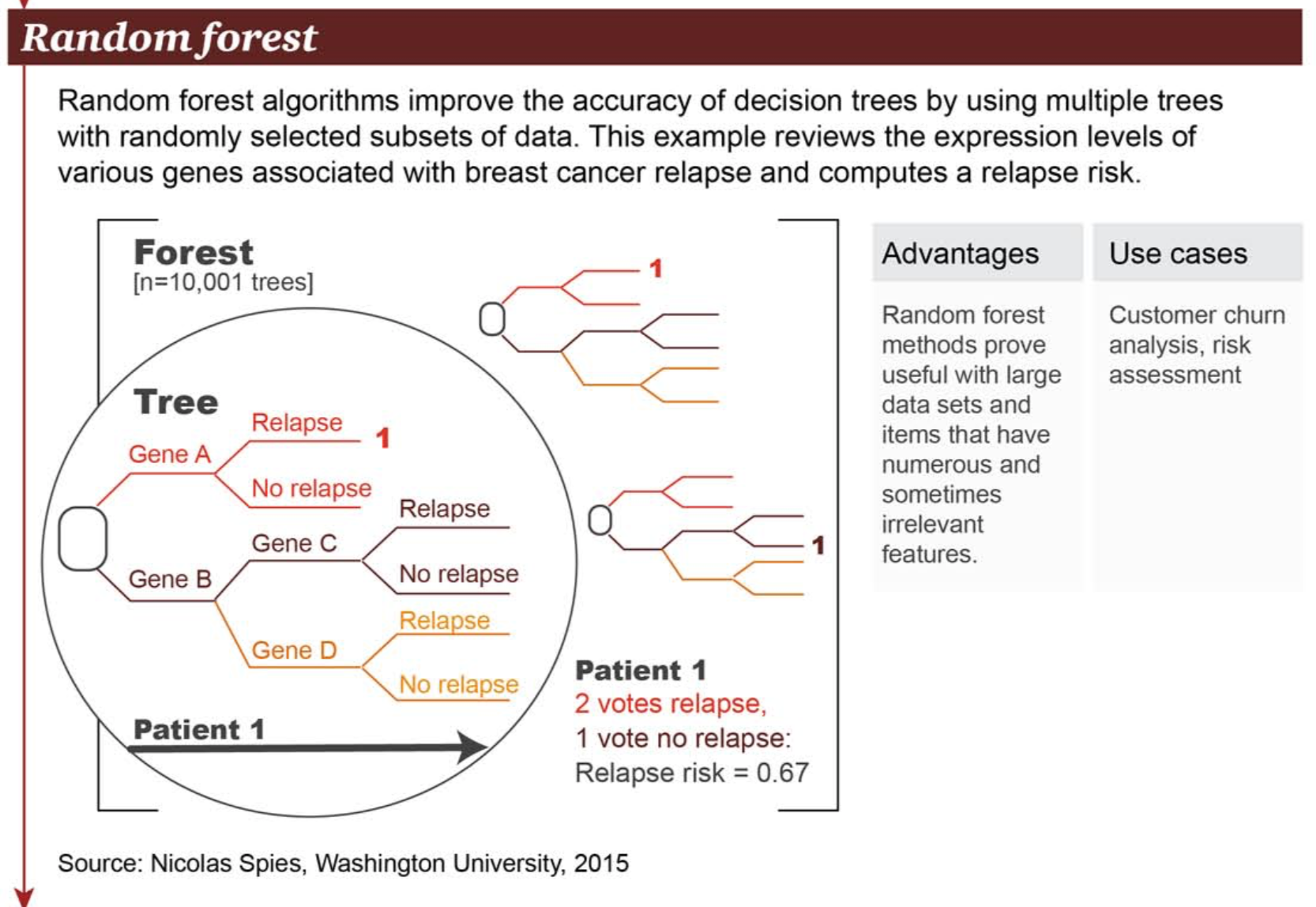
機器學習隨機森林
https://usblogs.pwc.com/emerging-technology/wp-content/uploads/2017/04/Machine_Learning_Twitter_2.png
乳腺癌復發風險評估
改良型決策樹
機器學習類神經網路
https://usblogs.pwc.com/emerging-technology/wp-content/uploads/2017/04/Machine_Learning_Twitter_2.png
循環式

深度學習類神經網路(1/14)

細胞核
樹突(接收訊號)
神經元細胞
髓鞘
施旺細胞
蘭氏結
突觸
軸突
(神經纖維,傳導)
輸入訊號
輸出訊號
深度學習類神經網路(2/14)
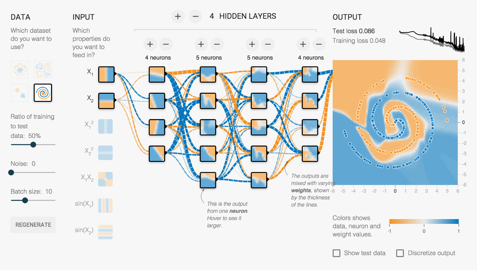
資料集
類神經網路(ANN)
輸入
隱藏層、神經元
輸出
深度學習Process(3/14)
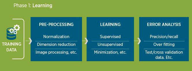
訓練資料
(學習階段)
資料前處理
學習
錯誤分析(含測試)
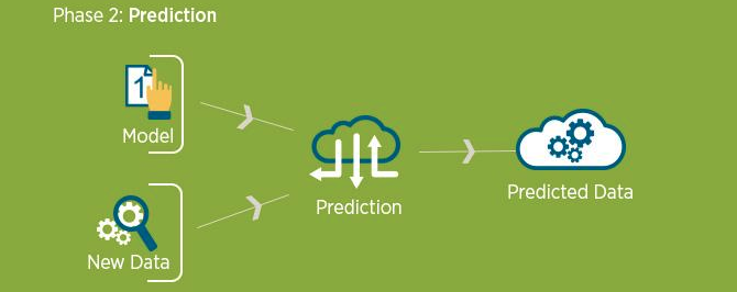
Model
(運用階段:預測)
新資料
驗證集
測試集
訓練集
預測
預測結果
深度學習
演算法
深度學習Process(4/14)
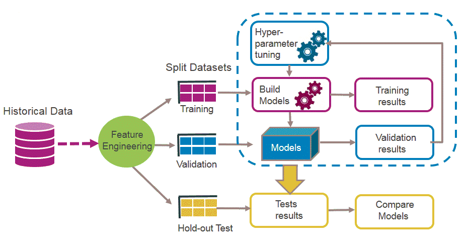
訓練資料
❶¹ 前處理
🅐 訓練集
🅑 驗證集
🅒 測試集
❷ 訓練參數
➎ 決定最終預測模型
❸ 產生預測用模型
➍ 測試模型
特徵萃取
❶² 資料集分割
深度學習Applications(5/14)
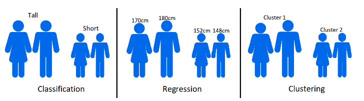
分類
迴歸
分群
- 三種常見應用
深度學習Applications(6/14)
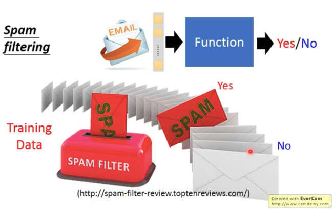
二元分類
- 分類(Classification)
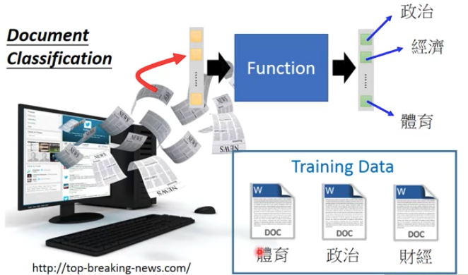
多元分類
深度學習Applications(7/14)

紀錄的關聯性
3種犯罪資料
歸納
較無偏差
盜竊,搶劫和大型殺戮:慣犯
傳統辦案:警察比對犯罪事件的特徵與記憶中的犯罪模式,篩出類似者並進一步調查
分類器
深度學習Applications(8/14)
濫用聊天功能
2019/4/11
辨識「惡意字眼」,較找出特定單字複雜得多

text selection engine
AI系統
❶ 偵測到可能惡意字眼

已確認/用戶未曾回報/無法辨識
知識模型
❷ 即時辨識
❸ 分類結果
❹ 人工處理
分類器
深度學習Applications(9/14)
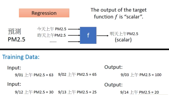
- 迴歸(Regression)
深度學習Applications(10/14)

4700萬人
投注85億美元
NCAA三月瘋

預測: 63場比賽勝負結果
迴歸
深度學習Applications(11/14)
機器學習預測競賽:
- 68隊 (8隊先打First Four) 67場 (68*67/2=2,278種組合) 的結果與機率

- 第一階段
- 第二階段
建立預測模型,回測2014~2018結果
送出2019的預測結果
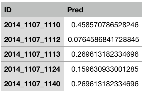
2014_隊伍1_隊伍2
隊伍1獲勝機率
迴歸
深度學習Applications(12/14)
應用領域
迴歸

訓練資料
病症: 癌症,心臟病,中風,糖尿病,關節炎,憂鬱症....
病人狀態: 血液,尿液和唾液樣本
預測死亡率
預測引擎
血液,尿液, 唾液樣本
病症
預防性措施

參考
醫囑
深度學習Applications(13/14)
- 分群(Clustering)
分類: 訓練資料有標記, 分群: 無標記
深度學習Applications(14/14)
2019/4/11
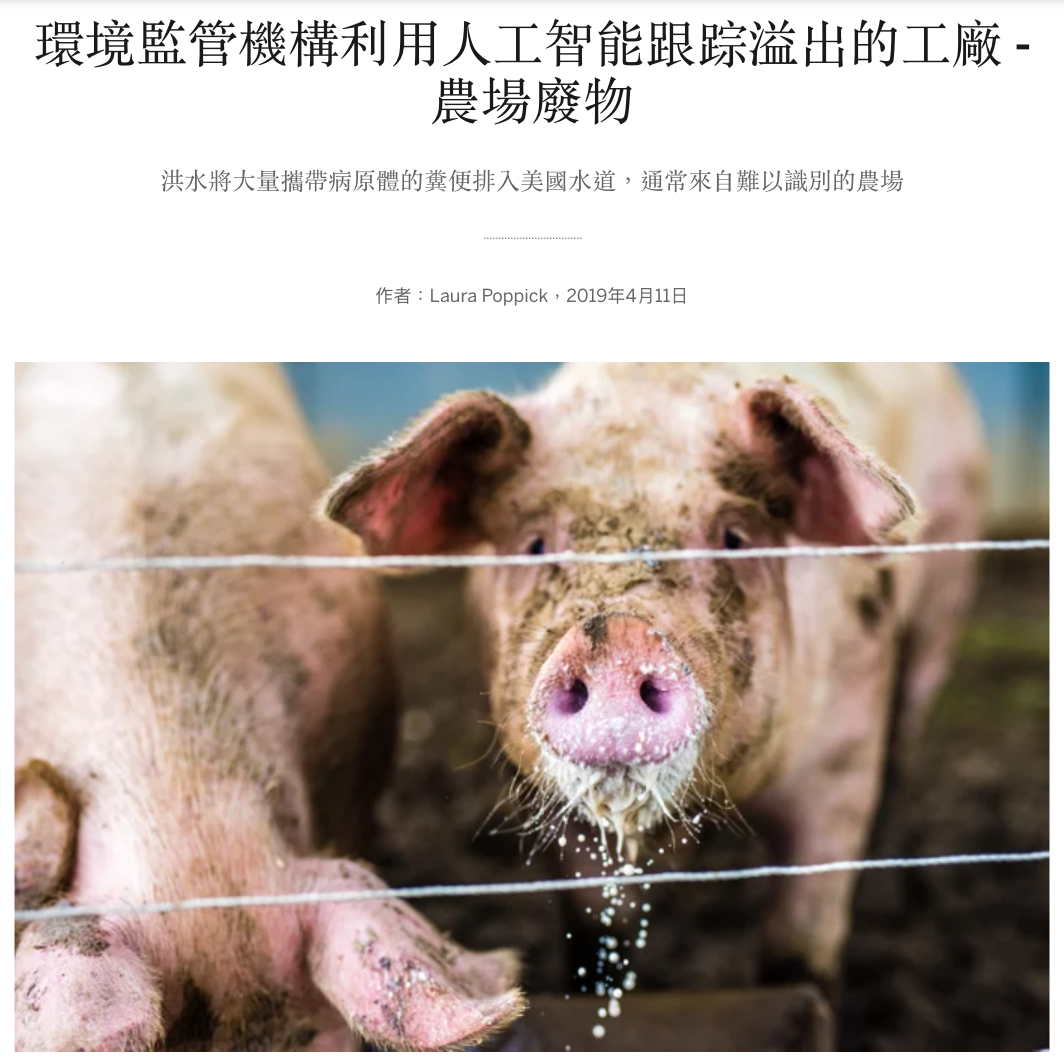
洪水將大量攜帶病原體的糞便排入水道,通常來自難以識別的農場
訓練資料
- 北卡: 24,440張衛星圖,手動標示農場特徵
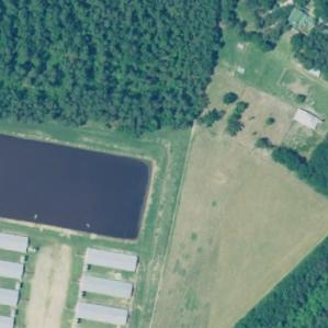
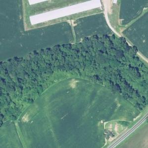
長而窄的建築群
潟湖
預測引擎
識別出農場的位置
新的衛星圖
分群
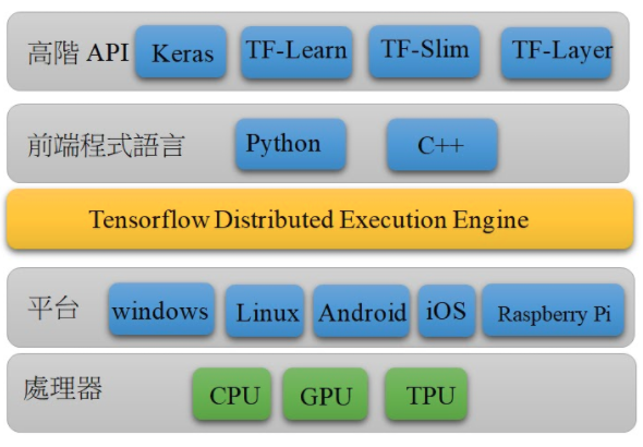
深度學習套件
Tensorflow
TensorFlow 架構
TensorFlow/Keras(R版本) (1/7)

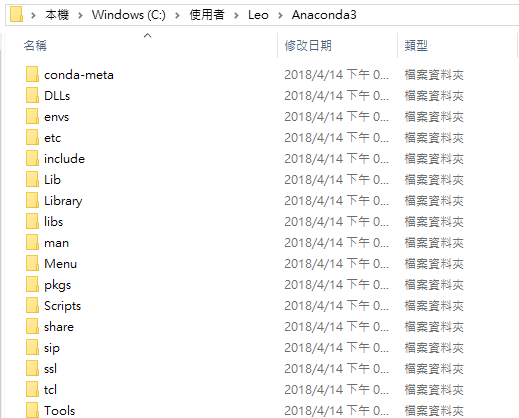
1. 安裝python環境:使用Anaconda包(Python 3.7版)
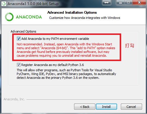
自動加入系統PATH變數
TensorFlow/Keras(R版本) (2/7)
2. 開啟Anaconda Prompt,創建r-tensorflow虛擬環境
conda create --name r-tensorflow python=3.7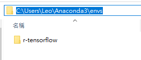
3. 在r-tensorflow環境裡,安裝tensorflow/keras
activate r-tensorflow
pip install --ignore-installed --upgrade tensorflow
conda install --channel defaults conda python=3.6 --yes
conda update --channel defaults --all --yes
conda install -c conda-forge keras
必須取名為r-tensorflow!!
(RStudio預設之讀取名稱)
TensorFlow/Keras(R版本) (3/7)
4. 測試tensorflow/keras是否安裝成功
activate r-tensorflow
python
- 進入python環境
import tensorflow as tf
hello = tf.constant('Hi, TensorFlow!')
session = tf.Session()
print(session.run(hello))- 輸入下列程式碼
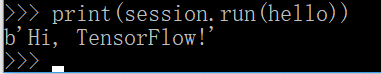
- 最後執行結果,成功!
TensorFlow/Keras(R版本) (4/7)
5. 安裝R, RTools與RStudio,並開啟RStudio
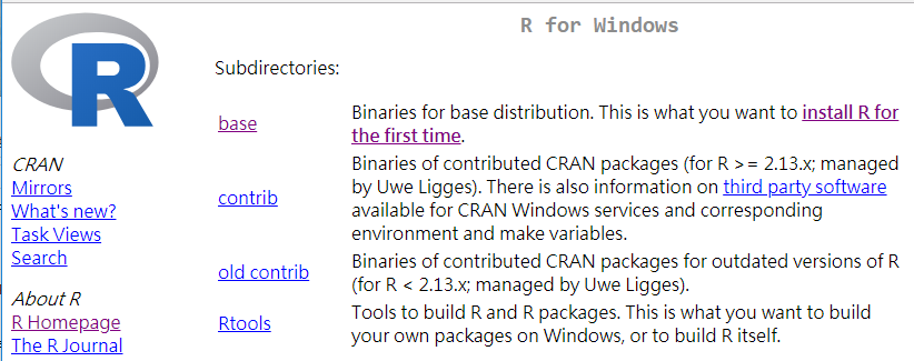
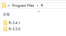
R安裝於Program Files
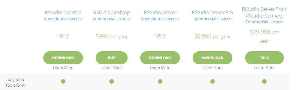
Desktop版
TensorFlow/Keras(R版本) (5/7)
6. 在RStudio內測試rstudio/tensorflow
```{r eval=FALSE}
# 安裝'devtools' package:方便從github安裝套件
if(!"devtools" %in% installed.packages())
  install.packages('devtools')

require(devtools)

# install tensorflow(如果你要tensorflow的話)
devtools::install_github("rstudio/tensorflow")

# installing keras(如果你要keras的話)
devtools::install_github("rstudio/keras")
```

```{r eval=FALSE}
# 測試tensorflow: Hello
require(tensorflow)
session = tf$Session()
hello <- tf$constant('Hi, TensorFlow!')
session$run(hello)
```
hello.rmd
TensorFlow/Keras(R版本) (6/7)
7. 在RStudio內測試rstudio/keras
```{r eval=FALSE}
library(keras)
model <- keras_model_sequential()
model %>%
  layer_dense(units = 256, activation = 'relu', input_shape= c(784)) %>%
  layer_dropout(rate = 0.4) %>%
  layer_dense(units = 128, activation = 'relu') %>%
  layer_dropout(rate = 0.3) %>%
  layer_dense(units = 10, activation = 'softmax')
summary(model)
```
keras.rmd
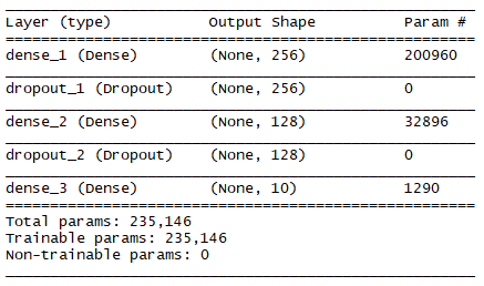
總共有235,146個可訓練參數!?
TensorFlow/Keras(R版本) (7/7)
R-Keras開發環境: 總整理

r-tensorflow

conda create --name r-tensorflow python=3.7
activate r-tensorflow
pip install -I -U tensorflow
conda install -c conda-forge keras


(R Rtools)

TensorFlow R
keras R
devtools::install_github("rstudio/tensorflow")
devtools::install_github("rstudio/keras")

library(keras)   ## Keras for R

❹
❶
❷
❸
❺
Keras model
Sequential model
Keras Model a simple approach
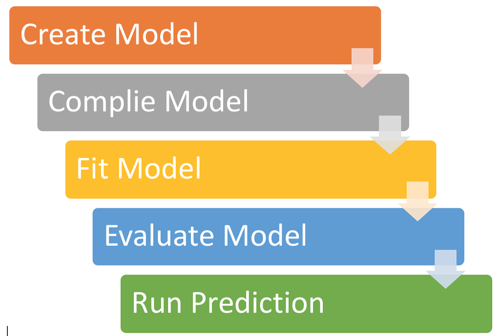
程式的階段
機器學習階段
訓練
測試
預測
建立模型
設定參數
訓練集
測試集
輸入層、隱藏層、輸出層
Keras Sequential Model (1/5)
```{r eval=FALSE}
library(keras)
model <- keras_model_sequential()
model %>%
  layer_dense(units = 256, activation = 'relu', input_shape= c(784)) %>%
  layer_dropout(rate = 0.4) %>%
  layer_dense(units = 128, activation = 'relu') %>%
  layer_dropout(rate = 0.3) %>%
  layer_dense(units = 10, activation = 'softmax')
summary(model)
```
keras.rmd
總共有235,146個可訓練參數!?
Keras Sequential Model (2/5)
model <- keras_model_sequential()
linear stack of layers
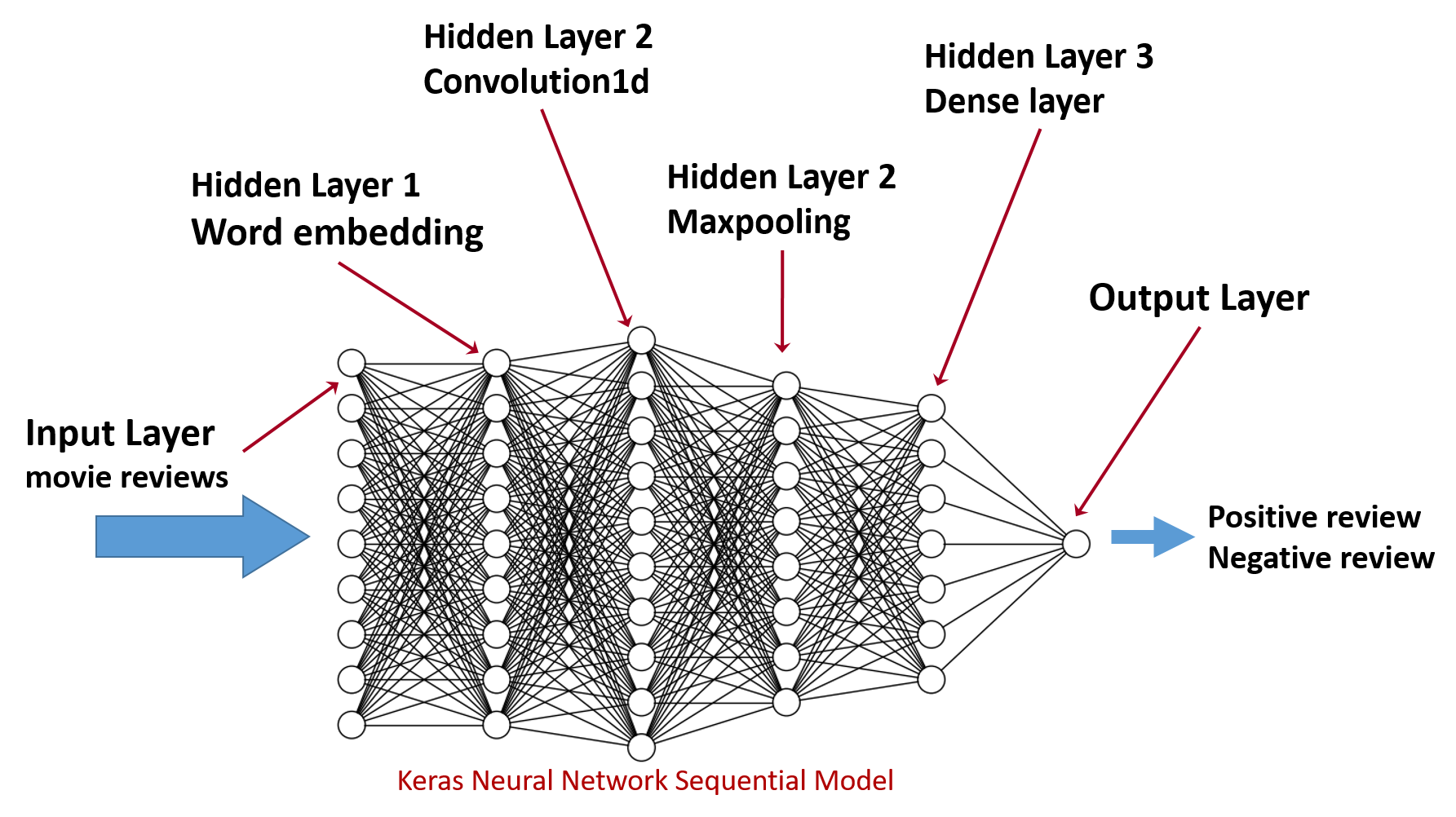
電影評論
情感分析
編碼: 建立向量
卷積: 萃取特徵
池化: 降低採樣
全連接層
Keras Sequential Model (3/5)

每一層可以有
1. 輸入資料
2. 權重(數量同該層的node數)
3. 激勵函數(activation function)
4. 輸入值的dropout機率
Keras Sequential Model (4/5)
  layer_dense(units = 256, activation = 'relu', input_shape= c(784)) %>%
  layer_dropout(rate = 0.4) %>%
784個值
784個值
256個節點
256個權重
dropout機率=0.4
relu函數
Keras Sequential Model (5/5)
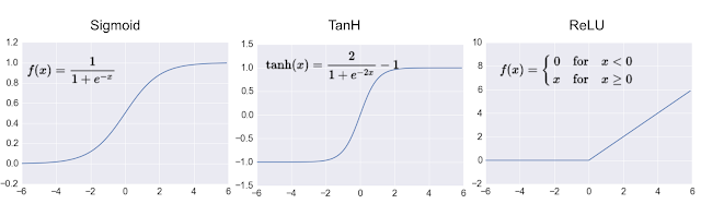
激勵函數類型
資料來源: http://www.cs.toronto.edu/~rsalakhu/papers/srivastava14a.pdf
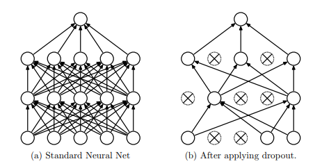
dropout效果
深度學習範例:MNIST
- 手寫辨識
- 資料集:MNIST dataset
MNIST資料集
訓練集:60000筆
測試集:10000筆
3維陣列(images筆數, 圖寬, 圖高)
圖:28*28 共784圖點

60000 rows
28 columns
.
.
.
28 slices
MNIST資料集檢視資料
1. 安裝 rstudio/keras, rstudio/tensorflow。
```{r eval=FALSE}
if(!"devtools" %in% installed.packages())
  install.packages("devtools");

if(!"keras" %in% installed.packages()) {
  require(devtools);
  install_github("rstudio/keras");
}
```
2. 下載mnist資料集。
```{r eval=FALSE}
# 準備資料集MNIST :手寫灰階圖片,每張圖28*28=784圖點
library(keras)
mnist <- dataset_mnist()   # 資料集內建於keras內
```
3. mnist資料集已分為訓練集與測試集,先檢視訓練集
```{r eval=FALSE}
# 資料集已分為訓練集/測試集
# $x: a 3-d array (images,width,height) of grayscale values
# $y: an integer vector with values ranging from 0 to 9
x_train_image <-mnist$train$x # 3D陣列,圖點集60000筆
x_train_image <- array_reshape(x_train_image, c(nrow(x_train_image), 784)) #轉成矩陣60000*784

y_train_label <-mnist$train$y # 整數vector,60000個答案

## 矩陣圖點旋轉函式,m--> matrix; 2-->apply to columns, rev function
rotate <- function(m) t(apply(m, 2, rev))
## sample函式
print_sample <- function(image, label, num) {
  if(num>0) {
    for( i in 1:num) {
      sample <- matrix(image[i,], nrow=28, ncol=28, byrow=TRUE)
      print(image(rotate(sample),sub=sprintf("答案: %s",label[i])))
    }
  }
}
## 列印訓練集前10筆
print_sample(x_train_image, y_train_label, 10)
```MNIST資料集檢視資料
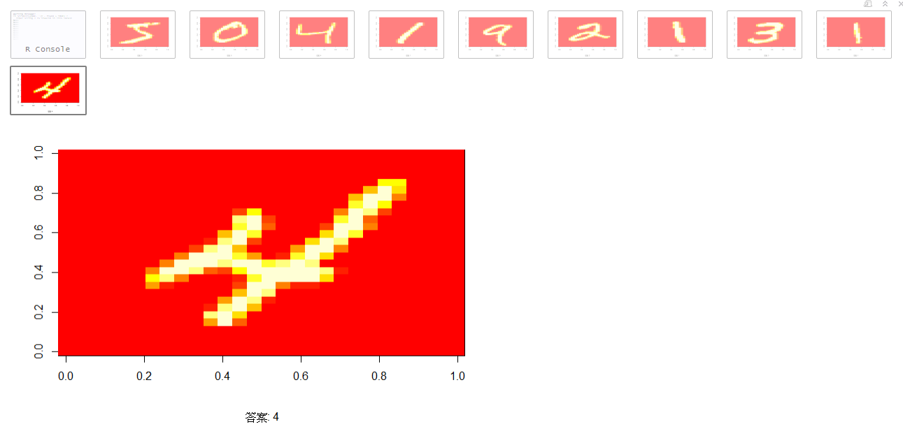
檢視前10筆
MNIST資料集前處理
```{r eval=FALSE}
if(!"devtools" %in% installed.packages())
  install.packages("devtools");

if(!"keras" %in% installed.packages()) {
  require(devtools);
  install_github("rstudio/keras");
}
```
下載mnist資料集。
```{r eval=FALSE}
# 準備資料集MNIST :手寫灰階圖片,每張圖28*28=784圖點
library(keras)
mnist <- dataset_mnist()   # 資料集內建於keras內
```
mnist資料集已分為訓練集與測試集,
```{r eval=FALSE}
# 資料集已分為訓練集/測試集
# $x: a 3-d array (images,width,height) of grayscale values
# $y: an integer vector with values ranging from 0 to 9
x_train_image <-mnist$train$x # 3D陣列,圖點集60000筆
x_train_image <- array_reshape(x_train_image, c(nrow(x_train_image), 784)) #轉成矩陣60000*784
x_test_image <-mnist$test$x
x_test_image <- array_reshape(x_test_image, c(nrow(x_test_image), 784))

y_train_label <-mnist$train$y # 整數vector,60000個答案
y_test_label <-mnist$test$y

```{r eval=FALSE}
# rescale: 將0~255數值轉成 0~1之間的整數
print(x_train_image[1,])
x_train_image <- x_train_image / 255
x_test_image <- x_test_image / 255
print(x_train_image[1,])

# 轉成matrix
print(y_train_label[1:10])
y_train_label <- to_categorical(y_train_label, 10)
y_test_label <- to_categorical(y_test_label, 10)
head(y_train_label,10)

```MNIST資料集前處理
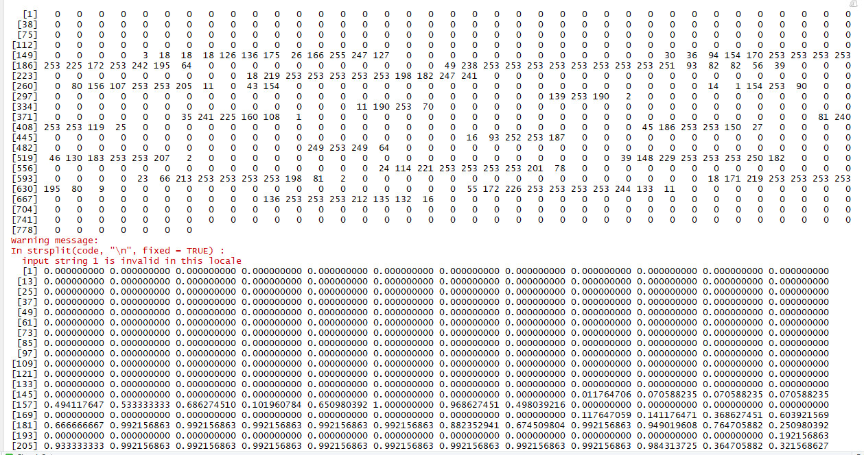
x_train_image, x_test_image
將0~255數值轉成 0~1之間的整數
MNIST資料集前處理
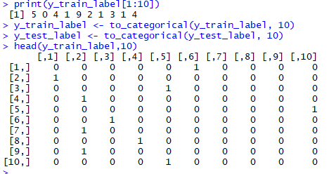
x_train_label由原來的向量,轉為60000*10的矩陣
第一筆的答案
MNIST資料集做法1:多層感知器
model <- keras_model_sequential()
MNIST資料集多層感知器:網路設定
model <- keras_model_sequential() #多元感知器
model %>%
  ## 輸入資料784個圖點
  layer_dense(units = 256, activation = 'relu', input_shape= c(784)) %>%
  layer_dropout(rate = 0.4) %>%
  layer_dense(units = 128, activation = 'relu') %>%
  layer_dropout(rate = 0.3) %>%
  ## 輸入資料10個數字機率
  layer_dense(units = 10, activation = 'softmax')
summary(model)
輸入層: 784個節點
layer_dense(units = 256, activation = 'relu', input_shape= c(784))隱藏層#1: 256個節點
layer_dense(units = 128, activation = 'relu')隱藏層#2: 128個節點
layer_dense(units = 10, activation = 'softmax')輸出層: 10個節點
MNIST資料集多層感知器:網路設定
輸入層: 784個節點
layer_dense(units = 256, activation = 'relu', input_shape= c(784))隱藏層#1: 256個節點
layer_dense(units = 128, activation = 'relu')隱藏層#2: 128個節點
layer_dense(units = 10, activation = 'softmax')輸出層: 10個節點
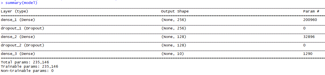
(784+1)*256=
(256+1)*128=
(128+1)*10=
MNIST資料集多層感知器:評估設定
## compile the model
model %>% compile(
  loss = 'categorical_crossentropy',
  optimizer = optimizer_rmsprop(),
  metrics = c('accuracy')
)
loss function: 評分公式
optimizer: 最佳化演算法
metrics: 評估效能的指標
MNIST資料集多層感知器:訓練階段
```{r eval=FALSE}
## 訓練階段
history <- model %>% fit(
  x_train, y_train,
  epochs = 30, batch_size = 128,
  validation_split = 0.2
)
plot(history)
epochs: 30次迭代(iterations)
batch_size: 取樣數量
validation_split: 驗證的案例比例為0.2,即20%(60000筆的20%為驗證案例, 80%為訓練案例)
MNIST資料集多層感知器:完整範例
```{r eval=FALSE}
# 準備資料集MNIST :手寫灰階圖片,每張圖28*28=784圖點
library(keras)
mnist <- dataset_mnist()   # 資料集內建於keras內

# 資料集已分為訓練集/測試集
# $x: a 3-d array (images,width,height) of grayscale values
# $y: an integer vector with values ranging from 0 to 9
x_train <-mnist$train$x
y_train <-mnist$train$y
x_test <- mnist$test$x
y_test <- mnist$test$y

rm(mnist)

#reshape: 3D array 轉成 2d matrix (圖1, 784個圖點)
x_train <- array_reshape(x_train, c(nrow(x_train), 784))
x_test <- array_reshape(x_test, c(nrow(x_test), 784))

# rescale: 將0~255數值轉成 0~1之間的整數
x_train <- x_train / 255
x_test <- x_test / 255

# 轉成matrix
y_train <- to_categorical(y_train, 10)
y_test <- to_categorical(y_test, 10)

```

```{r eval=FALSE}
##定義訓練模型
model <- keras_model_sequential()
model %>%
  ## 輸入資料784個圖點
  layer_dense(units = 256, activation = 'relu', input_shape= c(784)) %>%
  layer_dropout(rate = 0.4) %>%
  layer_dense(units = 128, activation = 'relu') %>%
  layer_dropout(rate = 0.3) %>%
  ## 輸入資料10個數字機率
  layer_dense(units = 10, activation = 'softmax')
summary(model)

## comple the model
model %>% compile(
  loss = 'categorical_crossentropy',
  optimizer = optimizer_rmsprop(),
  metrics = c('accuracy')
)

```
訓練與評估
```{r eval=FALSE}
## 訓練階段
history <- model %>% fit(
  x_train, y_train,
  epochs = 30, batch_size = 128,
  validation_split = 0.2
)
plot(history)

##測試階段
model %>% evaluate(x_test, y_test)

## 產生預測結果
model %>% predict_classes(x_test)
```
MNIST資料集多層感知器:訓練結果
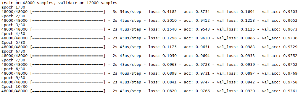
epochs: 30次迭代(iterations), 每次48000筆全數訓練完
batch_size: 128個案例, 故 1 epoch需跑375輪(48000/128)
acc: 訓練準確率
val_acc: 驗證準確率
MNIST資料集多層感知器:訓練結果
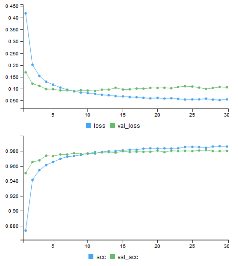
acc, val_acc 數值逐步提昇
30 epochs訓練驗證之後
acc為98.58%
val_acc為98%
MNIST資料集多層感知器:測試結果
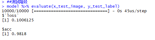
10000筆測試資料
測試正確率為 98.18%
訓練階段:acc為98.58%, val_acc為98%
MNIST資料集多層感知器:What's next?
1. 檢視「測試結果」中的錯誤案例
2. 了解是否需要修正model
model <- keras_model_sequential() #多元感知器
model %>%
  ## 輸入資料784個圖點
  layer_dense(units = 256, activation = 'relu', input_shape= c(784)) %>%
  layer_dropout(rate = 0.4) %>%
  layer_dense(units = 128, activation = 'relu') %>%
  layer_dropout(rate = 0.3) %>%
  ## 輸入資料10個數字機率
  layer_dense(units = 10, activation = 'softmax')
summary(model)
## comple the model
model %>% compile(
loss = 'categorical_crossentropy',
optimizer = optimizer_rmsprop(),
metrics = c('accuracy')
)## 訓練階段
history <- model %>% fit(
x_train, y_train,
epochs = 30, batch_size = 128,
validation_split = 0.2
)
plot(history)模型部署
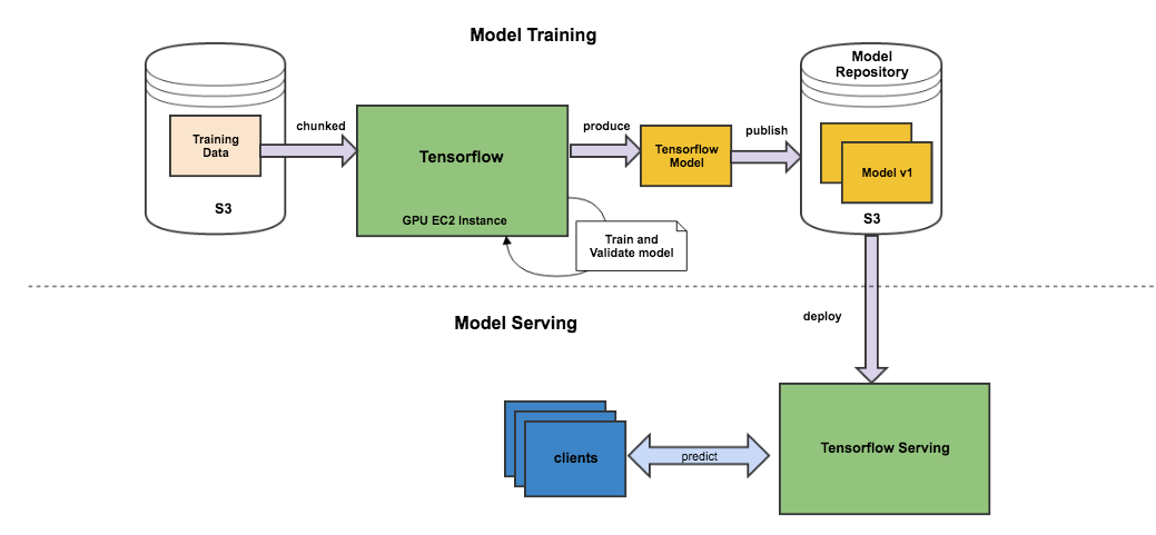
部署
模型部署
if(!"tfdeploy" %in% installed.packages()) {
  devtools::install_github("rstudio/tfdeploy")
}

library(tfdeploy)
export_savedmodel(model, "savemodel", remove_learning_phase = FALSE)
tfdeploy::serve_savedmodel("savemodel", browse = TRUE)
使用 rstudio/tfdeploy 套件
export_savedmodel(model, "資料夾名稱", remove_learning_phase = FALSE)
啟動REST 服務: http://localhost:8089
tfdeploy::serve_savedmodel("savemodel", browse = TRUE)模型部署新案例預測
{
  "instances": [
    {
      "image_input": [0.12,0,0.79,...,0,0]
    }
  ]
}
預測結果:
curl -X POST -H "Content-Type: application/json" -d @new_image.json http://localhost:8089/serving_default/predict準備好新圖檔new_image.json
{
  "predictions": [
    {
      "prediction": [ 1.3306e-24, 4.9968e-26, 1.8917e-23, 1.7047e-21, 0,
        8.963e-33, 0, 1, 2.3306e-32,2.0314e-22
      ]
    }
  ]
}
命令列測試: