A Study of the ISOMAP Algorithm and Its Applications in Machine Learning

Lucas Oliveira David

Universidade Federal de São Carlos

December 2015

Introduction

Machine Learning can help us with many tasks:

classification, estimation, data analysis and decision taking.

Data is an important piece of the learning process.

Visualization

Original Dermatology data set

Reduced Dermatology data set

D = [d]_{366 \times 34}

D = [d]_{366 \times 3}

Memory and Processing Time Reduction

Original Spam data set

S = [s]_{4601 \times 57}

2048.88 KB

Reduced Spam data set

107.84 KB

S = [s]_{4601 \times 3}

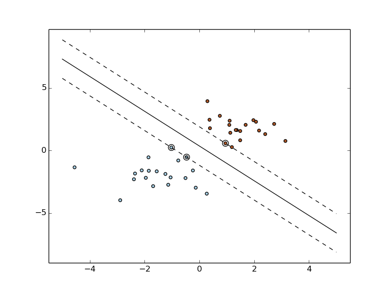
Data Preprocessing

Original R data set

(linearly separable).

Reduced R data set,

(still linearly separable).

Linear Dimensionality Reduction

Linear DR

Assumes linear distribution of data.
Combines features to create new components that point out the direction in which the data varies.
Sorts components by the variance.
Removes components with "small" variance.

(e.g., PCA, MDS)

PCA

Principal Component Analysis

1. Original data set.

2. Principal Components of K.

3. Basis change.

4. Component elimination.

PCA

\Sigma_X = \frac{1}{n} X^T X

X = U \Sigma V^T

\Sigma_X = \frac{1}{n} V \Sigma^2 V^T

Feature Covariance Matrix.

y = x V'

V is a change of basis orthonormal matrix.

Use V' to transform samples from X to Y.

y = x V

V' = sort(V, keys=|\lambda|)[0:d]

Find V', the base formed by the most important principal components.

SVD

MDS

Multidimensional Scaling

MDS

\Delta = [\delta_{rs}]_{n \times n} \mid \delta_{rs}^2 = \sum_i (x_{ri} -x_{si})^2

Pairwise distances.

B = -\frac{1}{2} H \delta^2 H = XX^T, X = U \Sigma^\frac{1}{2}

Full space reconstruction.

\begin{cases} \Sigma' = sort(\Sigma)[0:d] \\ U' = sort(U, keys=\Sigma)[0:d] \end{cases}

Sort eigenvalues and eigenvectors by

the value of the eigenvalues.

Y = U' \Sigma^{'\frac{1}{2}}

Embed it!

= x_r \cdot x_r + x_s \cdot x_s -2 x_r \cdot x_s

Nonlinear Dimensionality Reduction

Nonlinear DR

(e.g., ISOMAP, Kernel PCA)

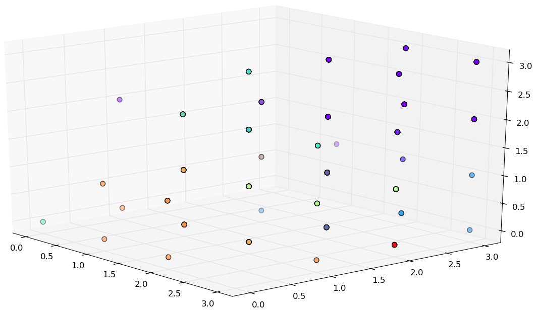
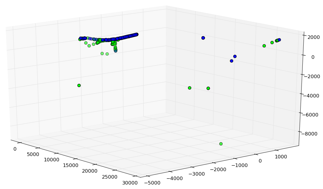
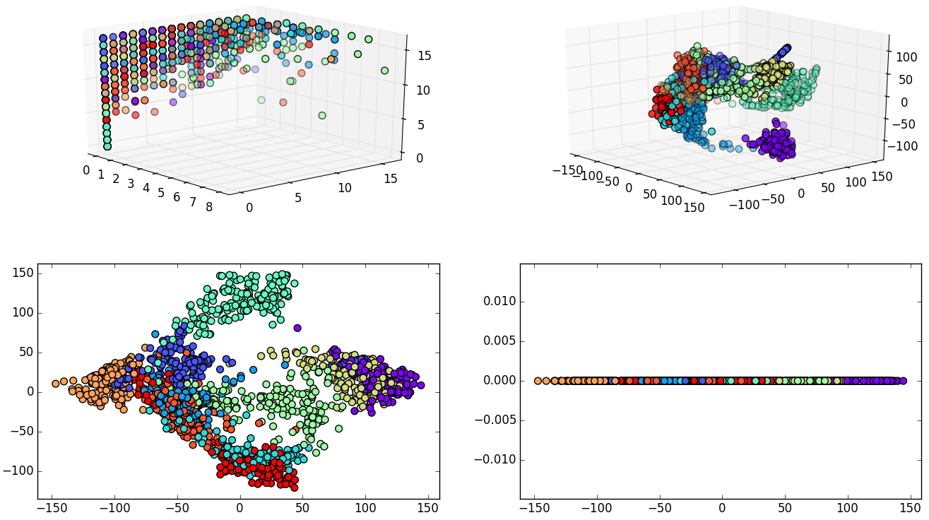
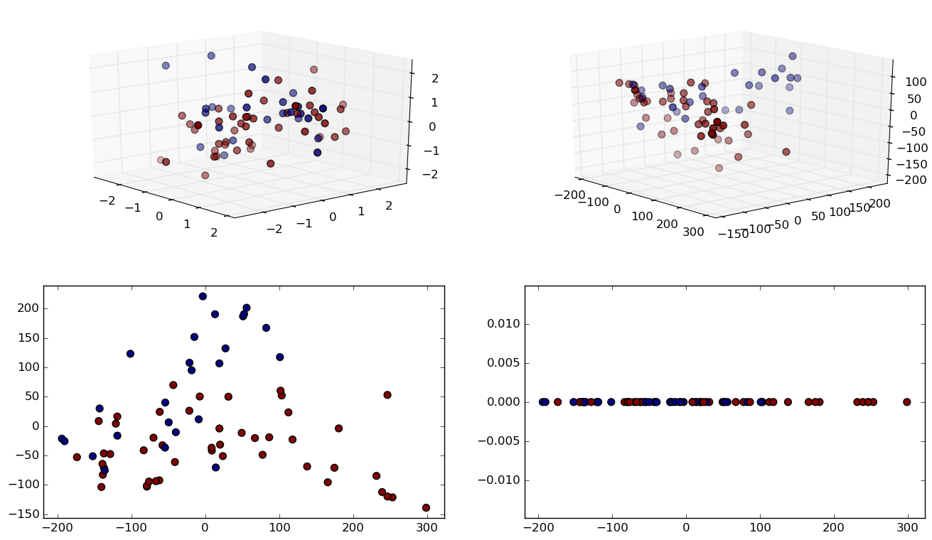
Q: what happens when data that follows a nonlinear distribution is reduced with linear methods?

A: very dissimilar samples become mixed as they are crushed onto lower dimensions.

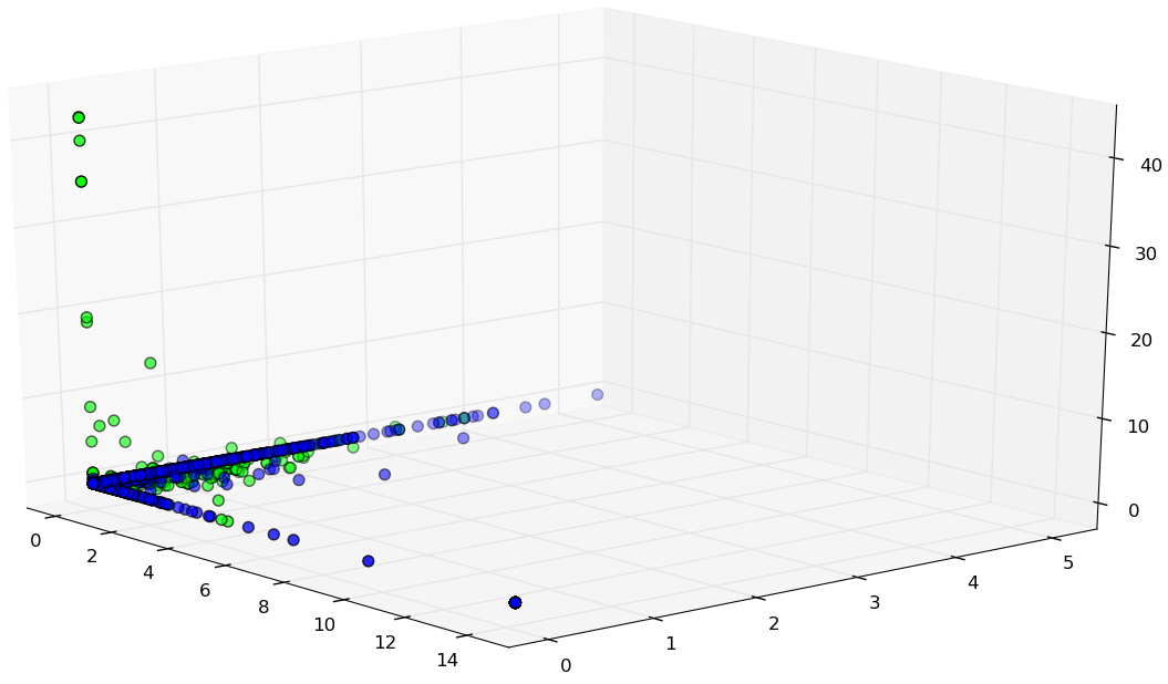
Nonlinear DR

Manifold Assumption.
Explores manifolds' properties such as local linearity and neighborhood.
Unfolding before reducing.

(e.g., ISOMAP, Kernel PCA)

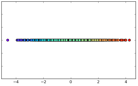
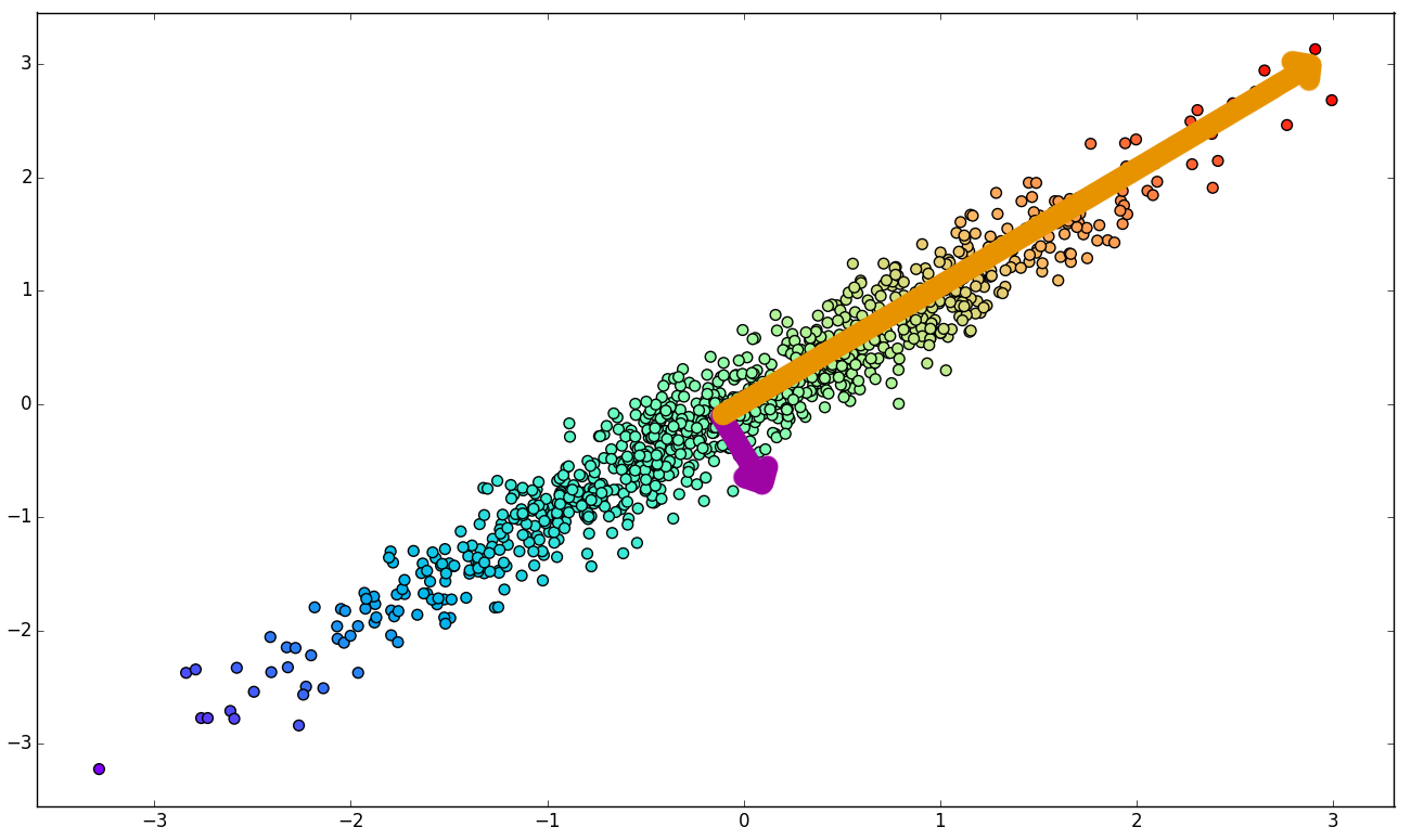
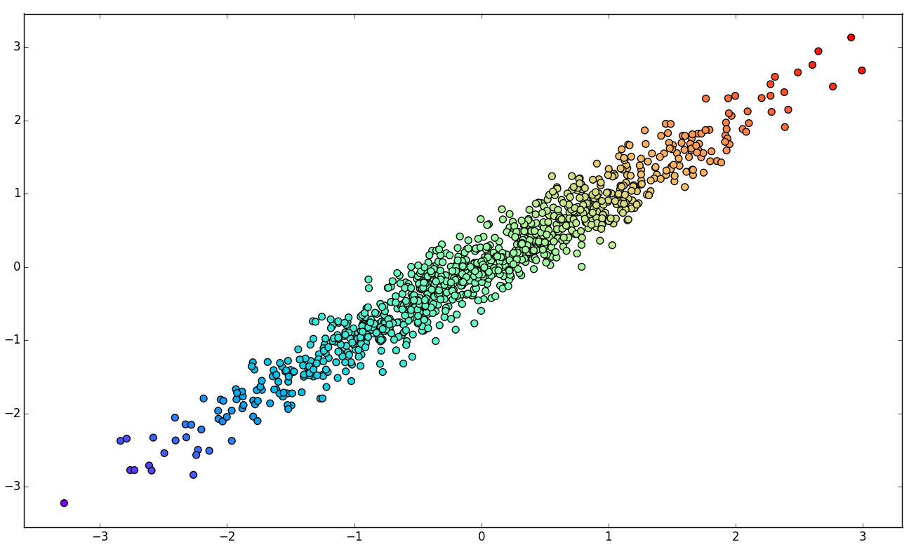
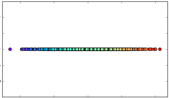
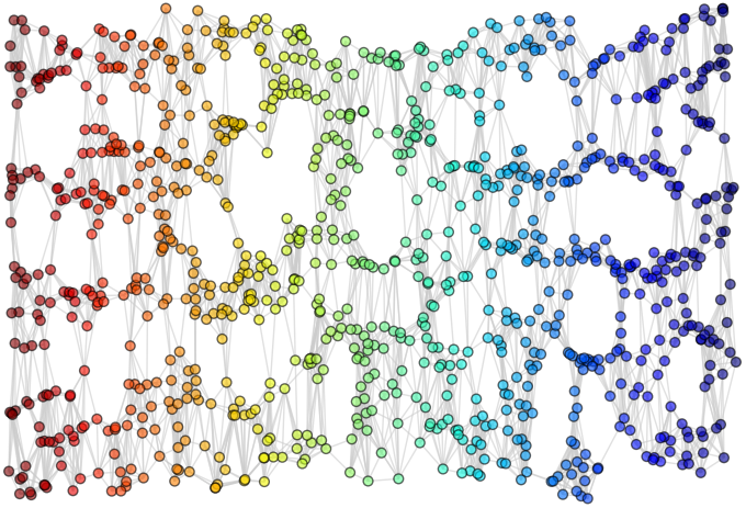
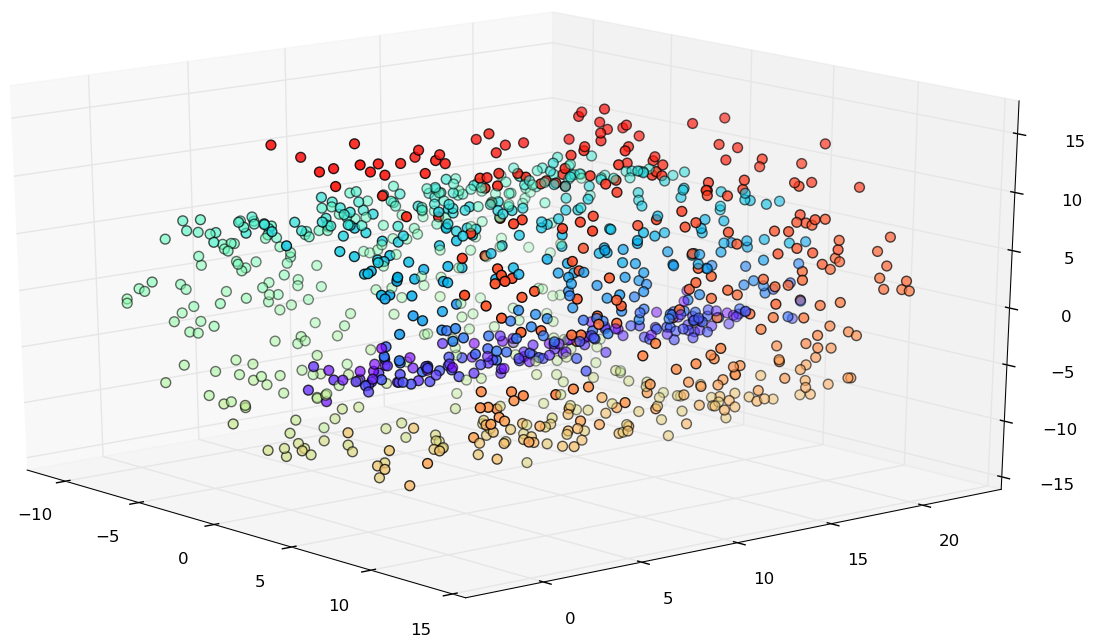
ISOMAP

Isometric Feature Mapping

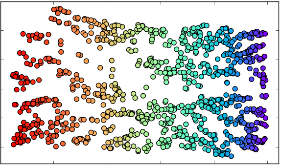
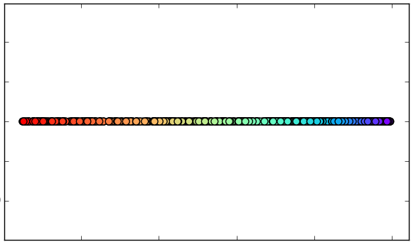
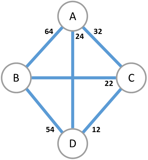
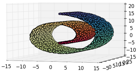
1. Original data set.

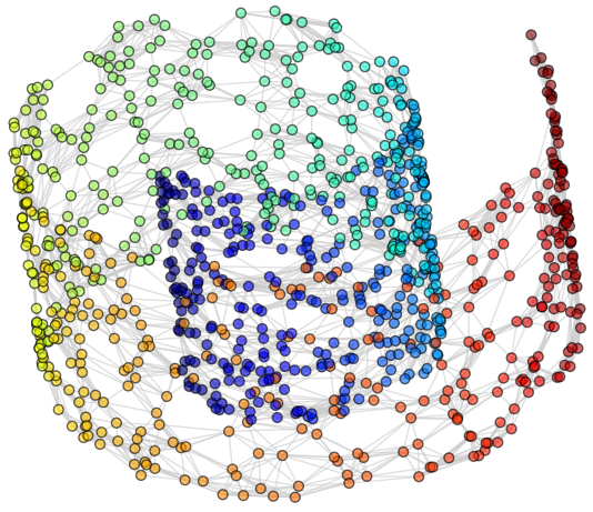
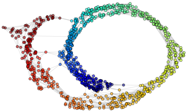
2. Compute neighborhood graph.

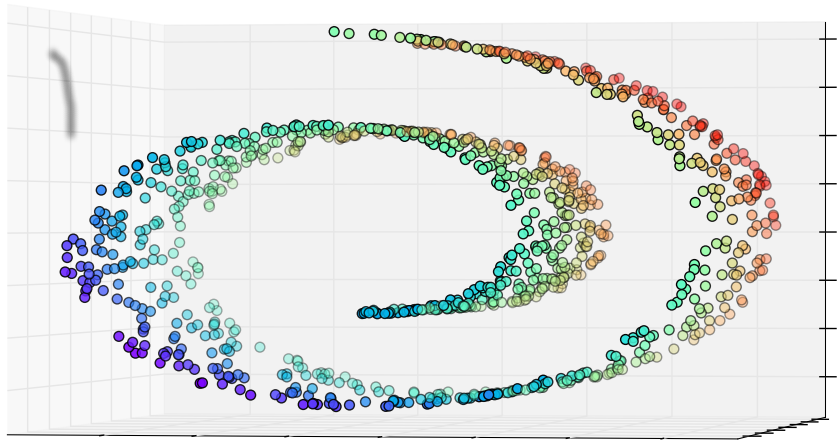
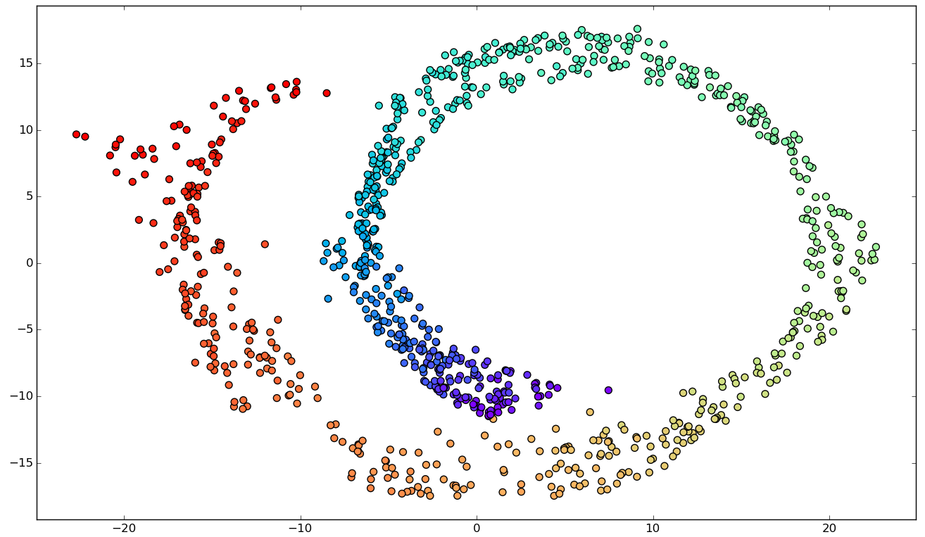
4.A. Reduction with MDS

(2 dimensions).

4.B. Reduction with MDS

(1 dimension).

\equiv

ISOMAP


def isomap(data_set, n_components=2,
           k=10, epsilon=1.0, use_k=True,
           path_method='dijkstra'):

    # Compute neighborhood graph.
    delta = nearest_neighbors(delta, k if use_k else epsilon)

    # Compute geodesic distances.
    if path_method == 'dijkstra':
        delta = all_pairs_dijkstra(delta)  
    else:
        delta = floyd_warshall(delta)

    # Embed the data.
    embedding = mds(delta, n_components)

    return embedding

ISOMAP

In Practice

ISOMAP In Practice

Experiment 1: Digits, 1797 samples and 64 dimensions.

Grid search was performed using a Support Vector Classifier.

	64 dimensions	10 dimensions
Accuracy	98%	96%
Data size	898.5 KB	140.39 KB
Grid time	11.12 sec	61.66 sec
Best parameters	'kernel': 'rbf', 'gamma': 0.001, 'C': 10	'kernel': 'linear', 'C': 1

54 dimensions eliminated with only 2% of accuracy loss.
It is also important to mention that grid search time has increased when the data dimensionality was reduced.

ISOMAP In Practice

Experiment 2: Leukemia, 72 samples and 7130 features.

ISOMAP In Practice

Grid search was performed using a Support Vector Classifier.

We observe massive memory requirement reduction, while loosing 11% of prediction accuracy.

ISOMAP In Practice

	7130 dimensions	10 dimensions
Accuracy	99%	88%
Data size	4010.06 KB	16.88 KB
Grid time	2.61 sec	.36 sec
Best parameters	'degree': 2, 'coef0': 10, 'kernel': 'poly'	'C': 1, 'kernel': 'linear'

ISOMAP's

Complexity

\text{1} \colon O(n^2)

\begin{cases} \text{2.A} \colon O[n^2(k + \log n)] \\ \text{2.B} \colon O[n^3] \end{cases}

\text{3} \colon O(n^3)


def isomap(data_set, n_components=2,
           k=10, epsilon=1.0, use_k=True,
           path_method='dijkstra'):

    # 1. Compute neighborhood graph.
    delta = nearest_neighbors(delta, k if use_k else epsilon)

    # 2. Compute geodesic distances.
    if path_method == 'dijkstra':
        delta = all_pairs_dijkstra(delta) # 2.A
    else:
        delta = floyd_warshall(delta)     # 2.B

    # 3. Embed the data.
    embedding = mds(delta, n_components)

    return embedding

Complexity

Reducing it to 3 dimensions took...

29.9 minutes, with my implementation.
10.76 seconds, with scikit-learn's!

Experiment 3: Spam, 4601 samples and 57 features.

Complexity

Obviously, we can do do better!

Studying scikit-learn's implementation:

Ball Tree is used for efficient neighbor search.
Shortest-path searches are implemented in C.
ISOMAP can be interpreted as the precomputed kernel for KernelPCA.
- ARPACK is used for the eigen-decomposition.
Many of the steps can be parallelized.

-\frac{1}{2}H \delta^2 H

Extensions

ISOMAP as Kernel PCA

\Sigma_X = \frac{1}{n} X X^T

"Kernel Trick"

\Sigma_{X_{ij}} = \frac{1}{n} K(x_i, x_j) = \frac{1}{n} \phi(x_i) \phi(x_j)^T

Sample Covariance Matrix.

Extensions

L-ISOMAP

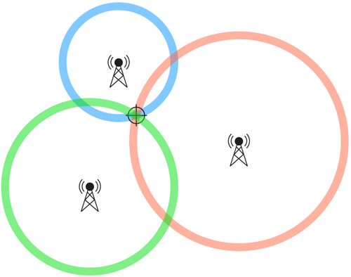
In a n-dimensional space with N samples, a point's position can be found from its distance to n+1 landmarks and their respective position.

Calculates the dissimilarity matrix
Apply MDS to the sub-matrix
Embed the rest of the data using the eigenvectors found.

[\delta]_{n \times N}

[\delta]_{n \times n}

Limitations

Manifold Assumption

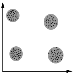
Disconnected graphs.

Incorrect reductions.

Possible work-around: increasing the parameters k or epsilon.

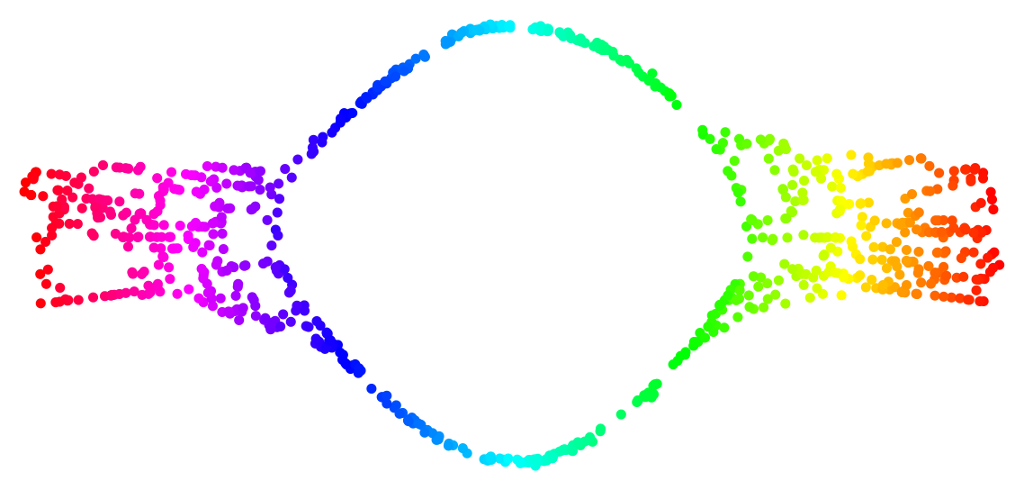
Limitations

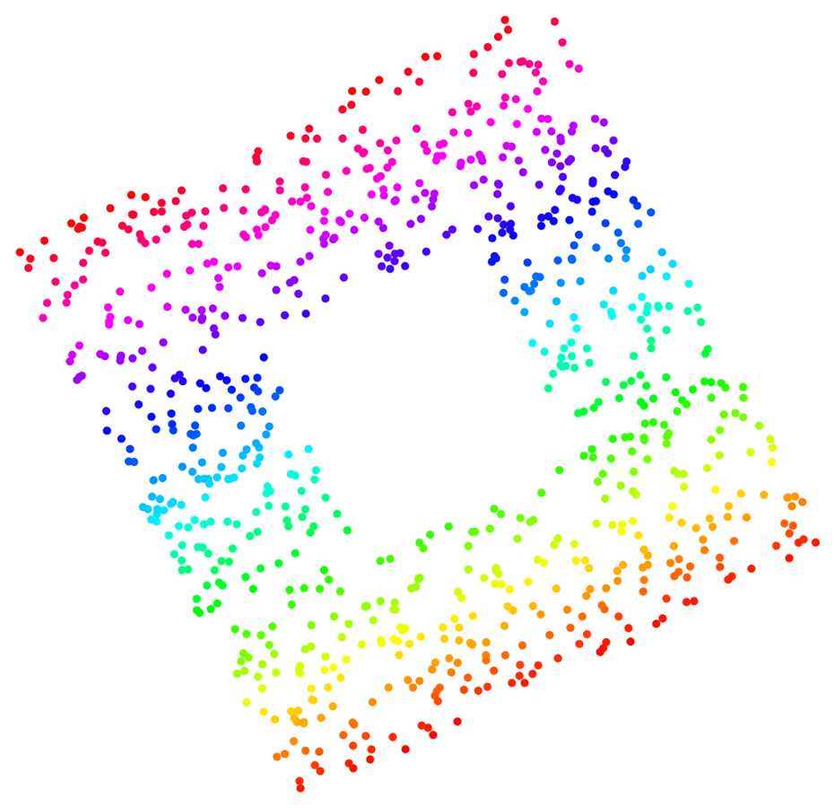
Manifold Convexity

Deformation around the "hole".

Limitations

Noise

Incorrect unfolding.

Possible work-around: reducing the parameters k or epsilon.

Final Considerations

ISOMAP performed well on many experiments.
However, it makes serious assumptions and it has its limitations. It is hard to say how it will behave on real-world data.
ISOMAP is a landmark on Manifold Learning.

Thank you if you made it this far!

For ISOMAP implementation and experiments, check out my github: github.com/lucasdavid/manifold-learning.