Investor Attention and the Cross-section of Analyst Coverage
Charles Martineau and Marius Zoican
Bank of Lithuania
October 16, 2020

Motivation
Analyst coverage across stocks (2017Q4)
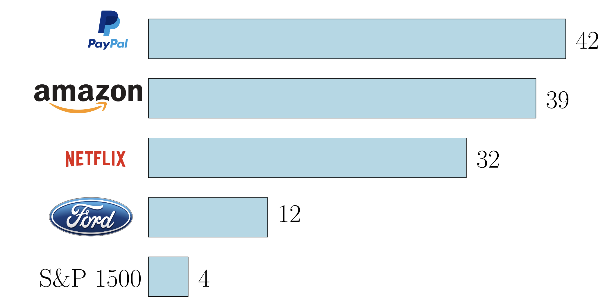
What drives the demand for information?
- Investors need information to choose portfolios.
- Limited attention can lead to suboptimal investment decisions:

- Portfolio under-diversification
- Home bias
What drives the supply for information?
- A key source of information comes from equity analysts, who disseminate financial information through reports.

How does investor attention impact analyst coverage choices?
Analyst objective
Maximize trading volume & revenue for brokerage house.
(Groysberg, Healy, and Maber, 2011)
Research question
This paper
- Empirical: How much does investor attention matter for analyst coverage choices?
- Theory: Build a noisy REE model to understand how attention constraints drive analyst coverage.
Contributions
Results
- Investor attention explains 21.52% of cross-sectional variation in analyst coverage -- second only to firm size.
- Model predicts coverage clustering, consistent with the data.
- Coverage clustering first , then in attention capacity.
- Relaxing cognitive constraints may not lead to more balanced coverage.
Literature
A growing literature shows that investor attention plays an important role in asset pricing at determining, e.g.,:
- price efficiency (Hirshleifer and Teoh, 2009)
- risk premium (Andrei and Hasler, 2015)
- return predictability (Da, Engelberg, and Gao, 2011)
- comovement (Peng and Xiong, 2006)
However, we know little on how investor attention influence information supply in financial markets.
Empirical results
A measure of attention
- Bloomberg provides a daily score, ranging from 0 to 4, to reflect the (abnormal) investor attention.

- We follow Ben-Rephael, Da, and Israelsen (2017).
- The score measures the number of times terminal users actively search and read articles about a particular stock.
- We collect the score between 2012-2017 and take yearly averages.
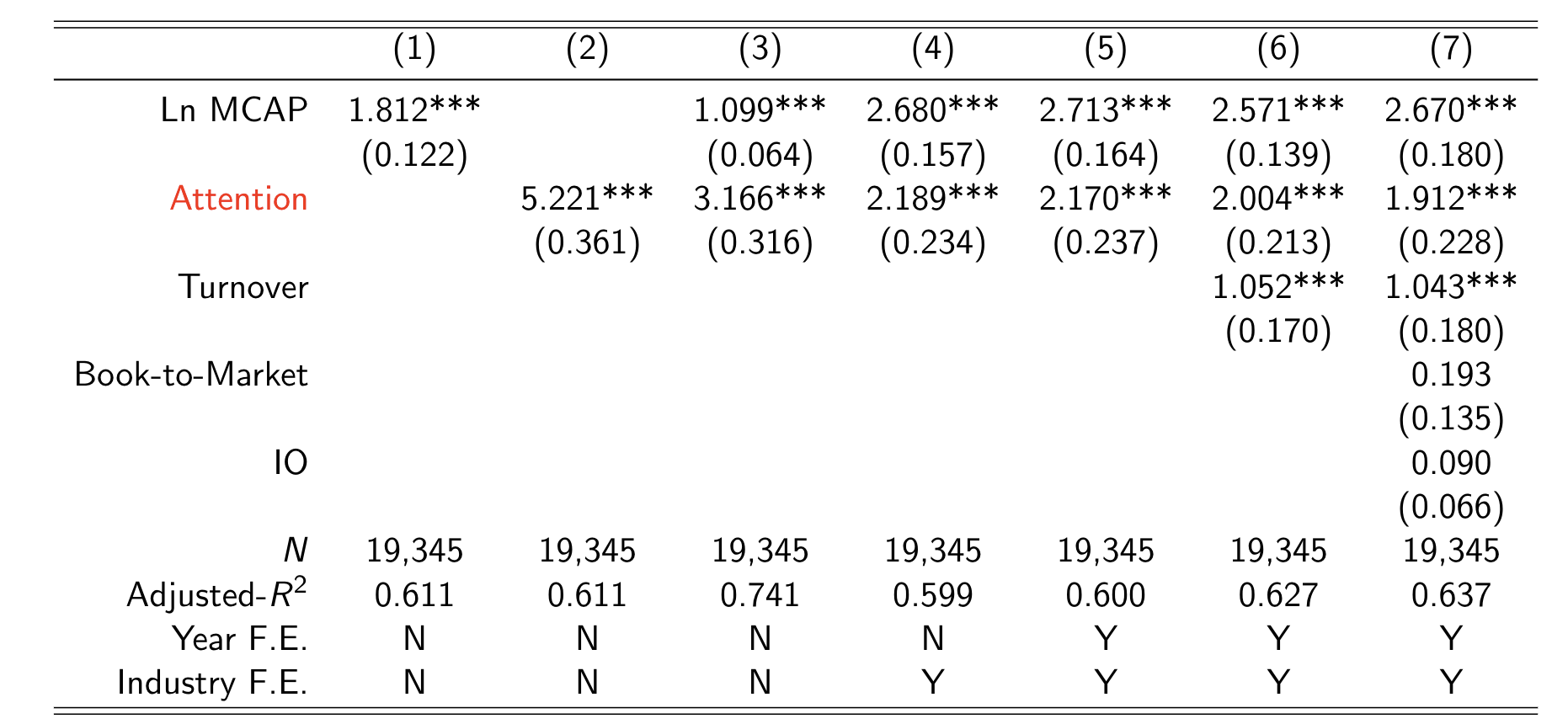
Investor attention and analyst coverage
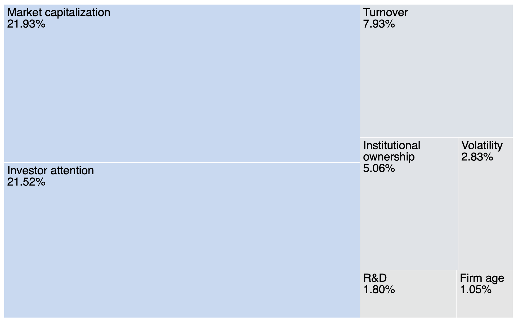
*using Shapley-Owen decomposition
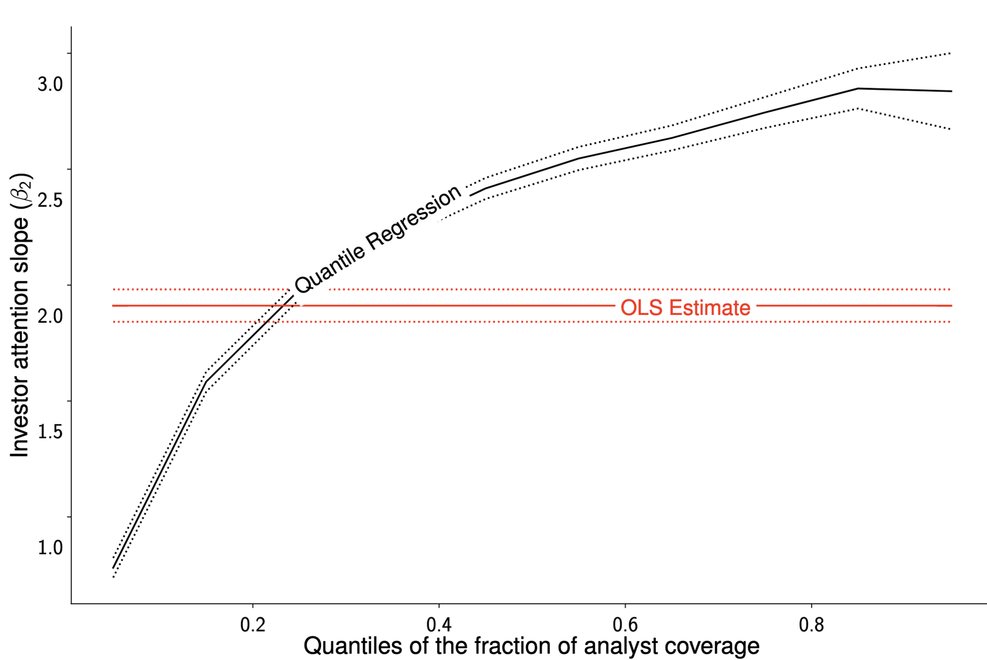
Analysts are more sensitive to attention for well-covered stocks
Model
Model ingredients
Assets
Two risky-assets in zero net supply, paying off at t=2
1. A high-precision asset H:
2. A low-precision asset L:
- Continuum of investors I with unit endowment and CARA preferences:
- Noise traders (i.i.d. across stocks) with variance
- Two analysts (k) who provide a public signal for one asset:
Agents
Investor attention and learning
Each investor j can acquire unbiased signals about stock i:
Investors choose the signal precision, but have finite learning (attention) capacity K:
Learning cost is lower if more analysts cover stock i
(through a "familiarity" argument):
(note decreasing returns to scale)
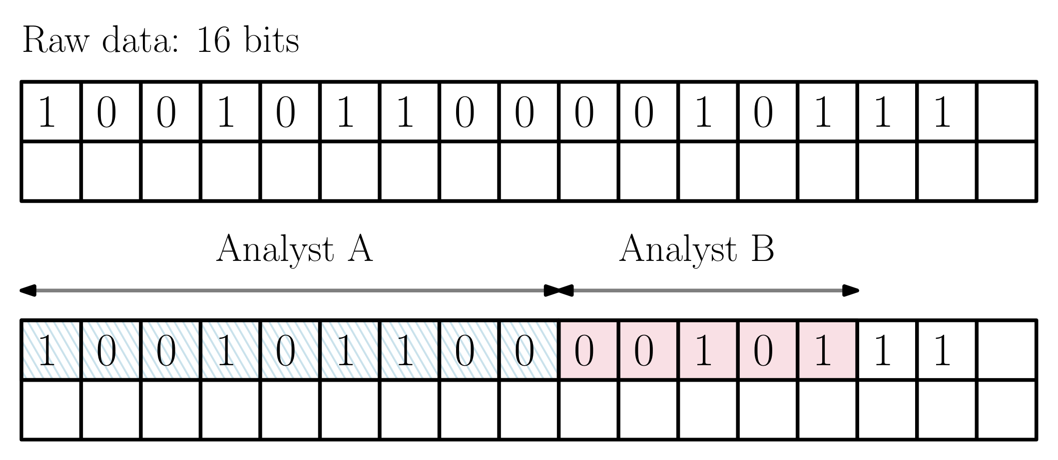
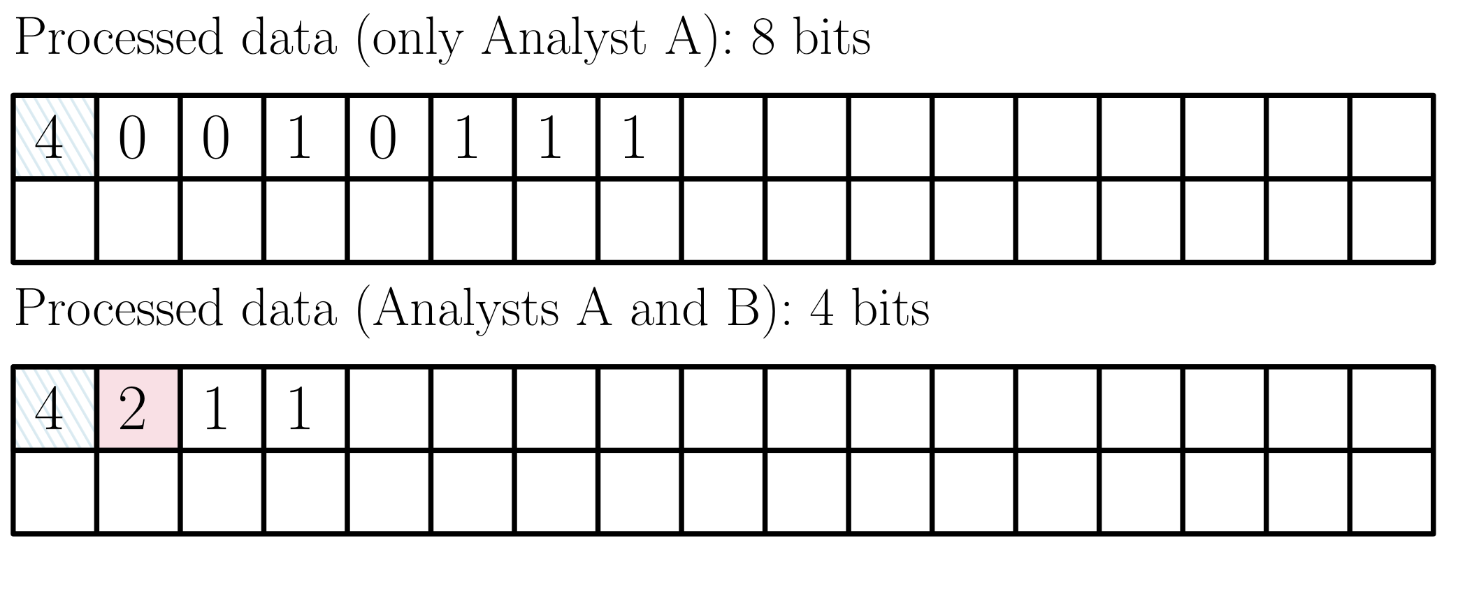
Analyst coverage as data compression
Analyst coverage as data compression

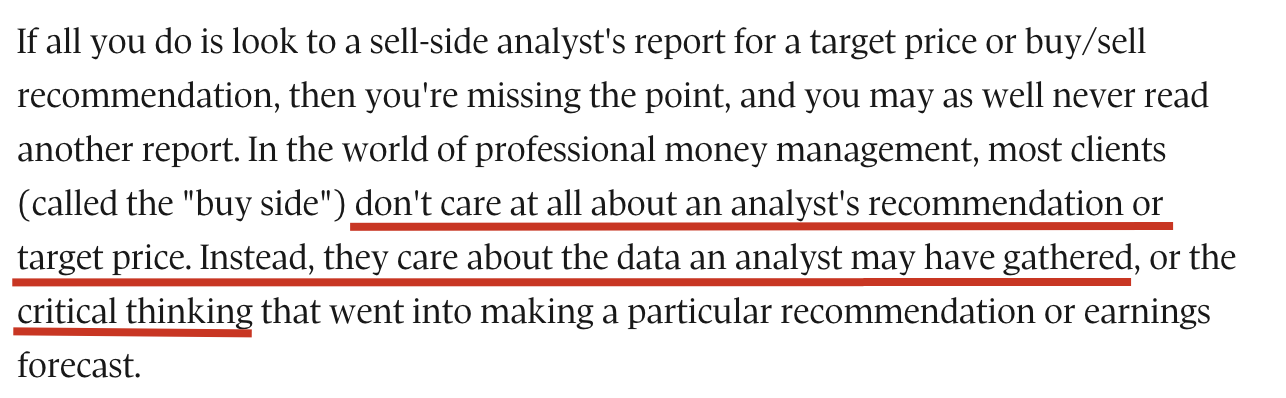
Analyst objective
- Sell-side analysts work for brokerage houses.
- Brokerage houses charge a fee f per unit of traded volume.
- Therefore, analysts choose to cover stocks to maximize expected volume for their brokerage house:
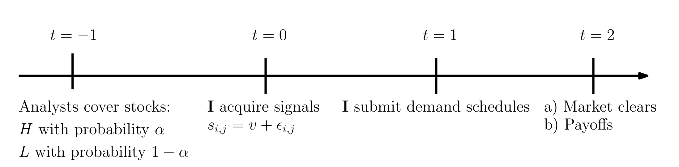
Model timing
Solving for equilibrium: Market clearing
(i) Conjecture linear price:
(ii) Optimal demand from investor j, conditional on signal:
(iii) Market clearing condition:
(iv) Clearing price:
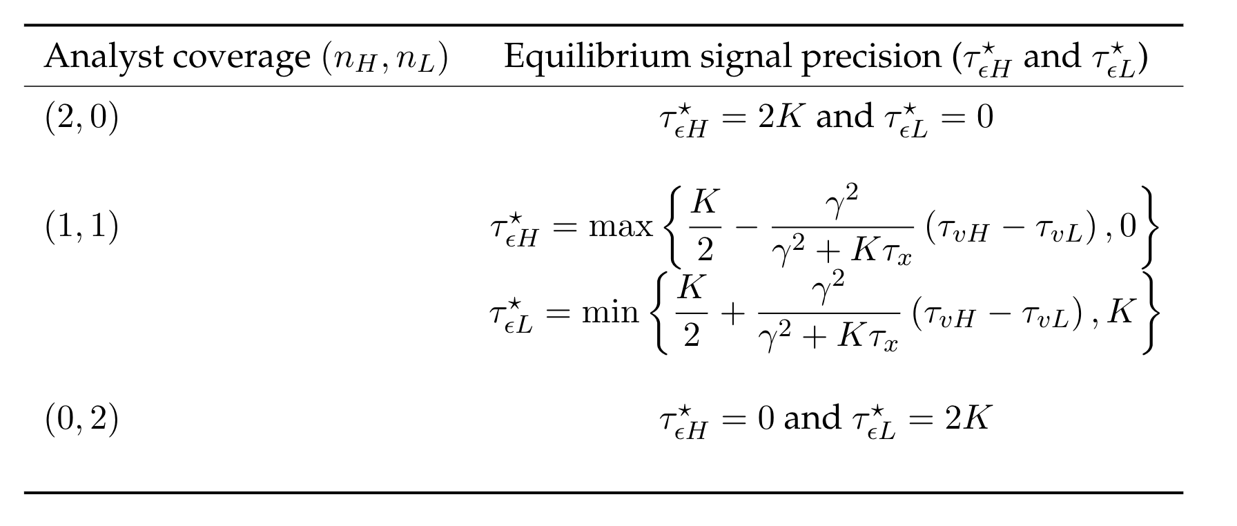
Solving for equilibrium: Private signals
Following Verrecchia (1982), problem boils down to:
Posterior precision
A measure of price impact
Investors have zero mass so take price as given.
Problem becomes:
Text
Attention constraint
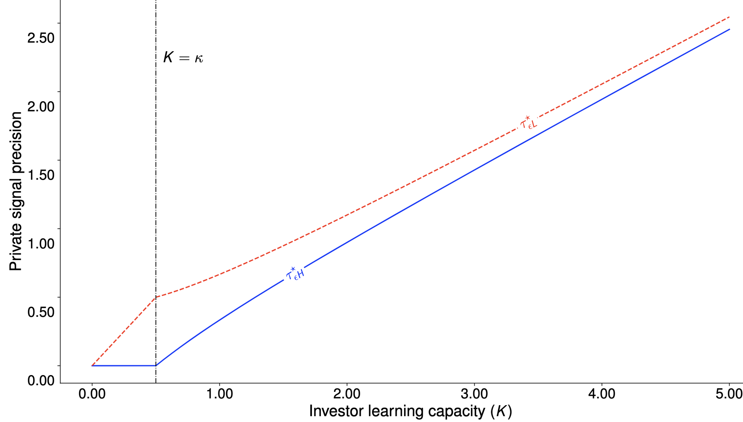
Investors only learn about H if capacity is large enough
Optimal signal acquisition and coverage
Solving for equilibrium: analysts' problem
The expected volume in a given stock i is:
Mechanism
- Coverage Private learning Confidence in signal Volume
- Public forecasts are common knowledge influence prices, but not volumes.
Analyst choice
If analyst j covers stock H, her utility is:
If analyst j covers stock H, her utility is:
If analyst j covers stock L, her utility is:
The equilibrium probability to cover stock H is:
Equilibrium analyst coverage distribution
Coverage odds-ratio can exceed risk odds-ratio
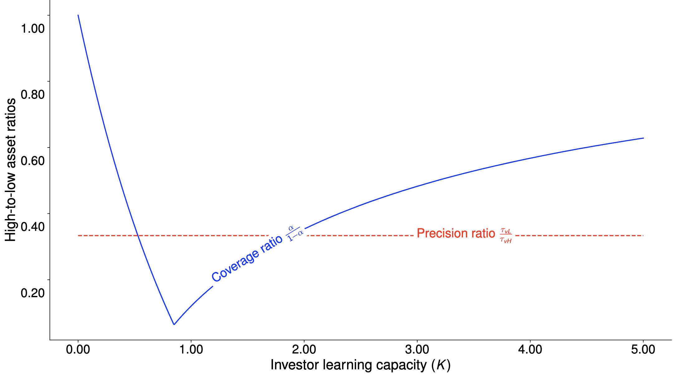
Example: If stock L has a payoff variance 3x that of stock $H$, it can have up to 10x more analyst coverage in expectation
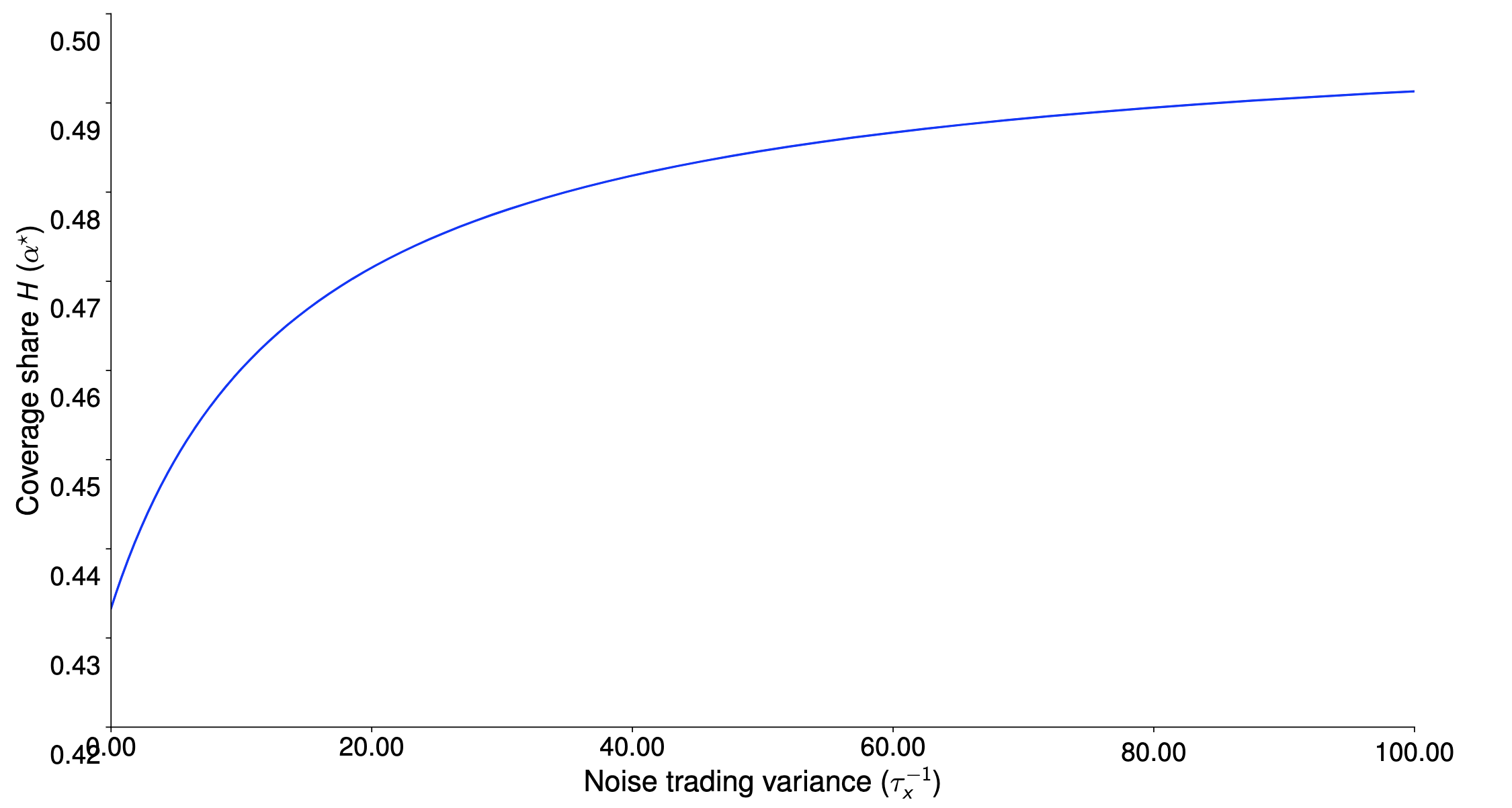
Analyst coverage and noise trading
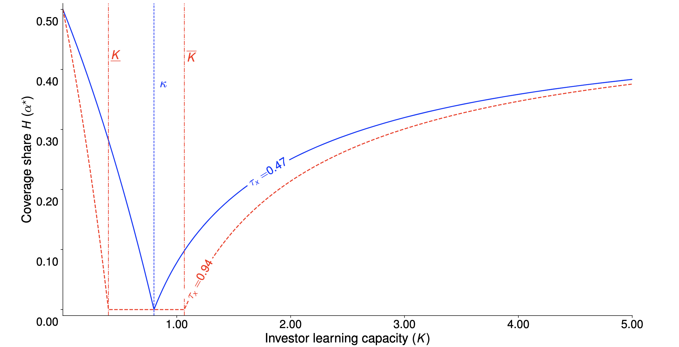
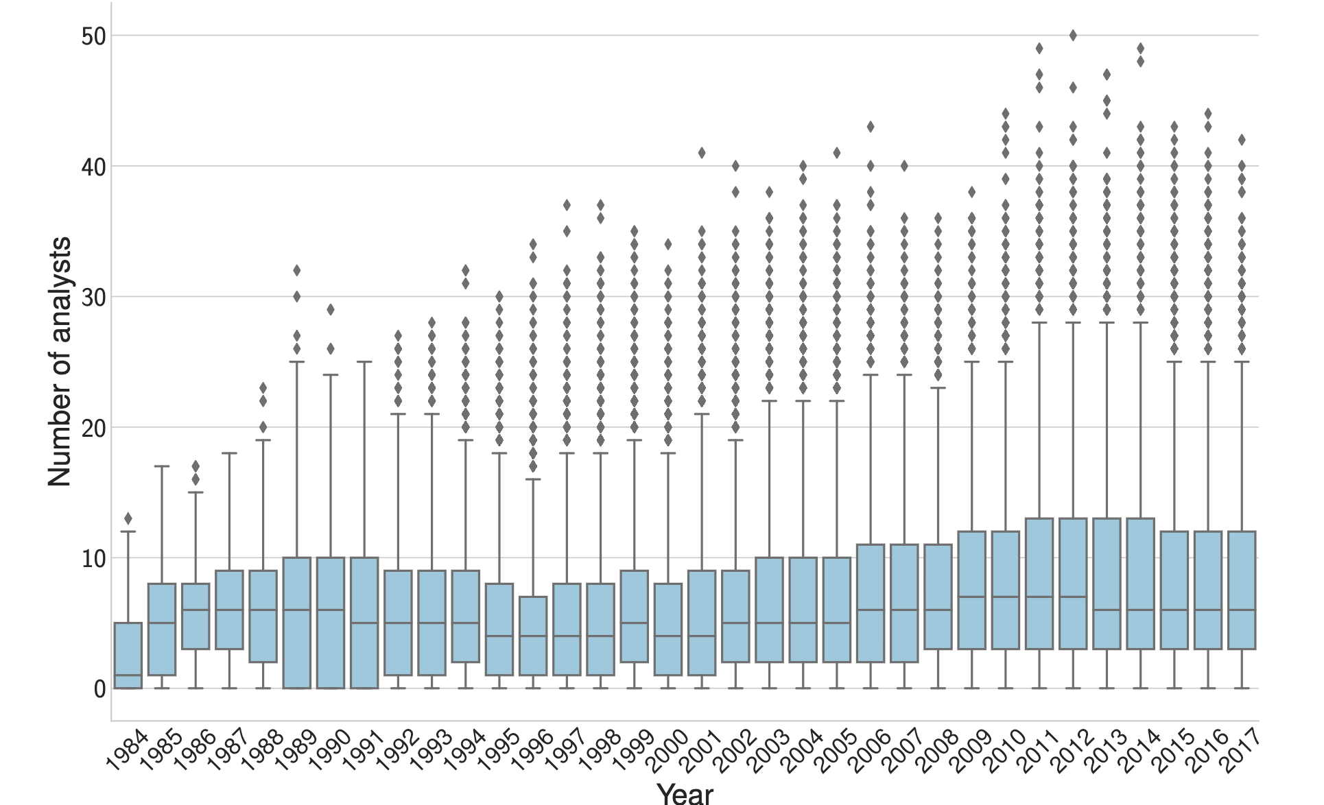
Coverage clustering
empirical evidence
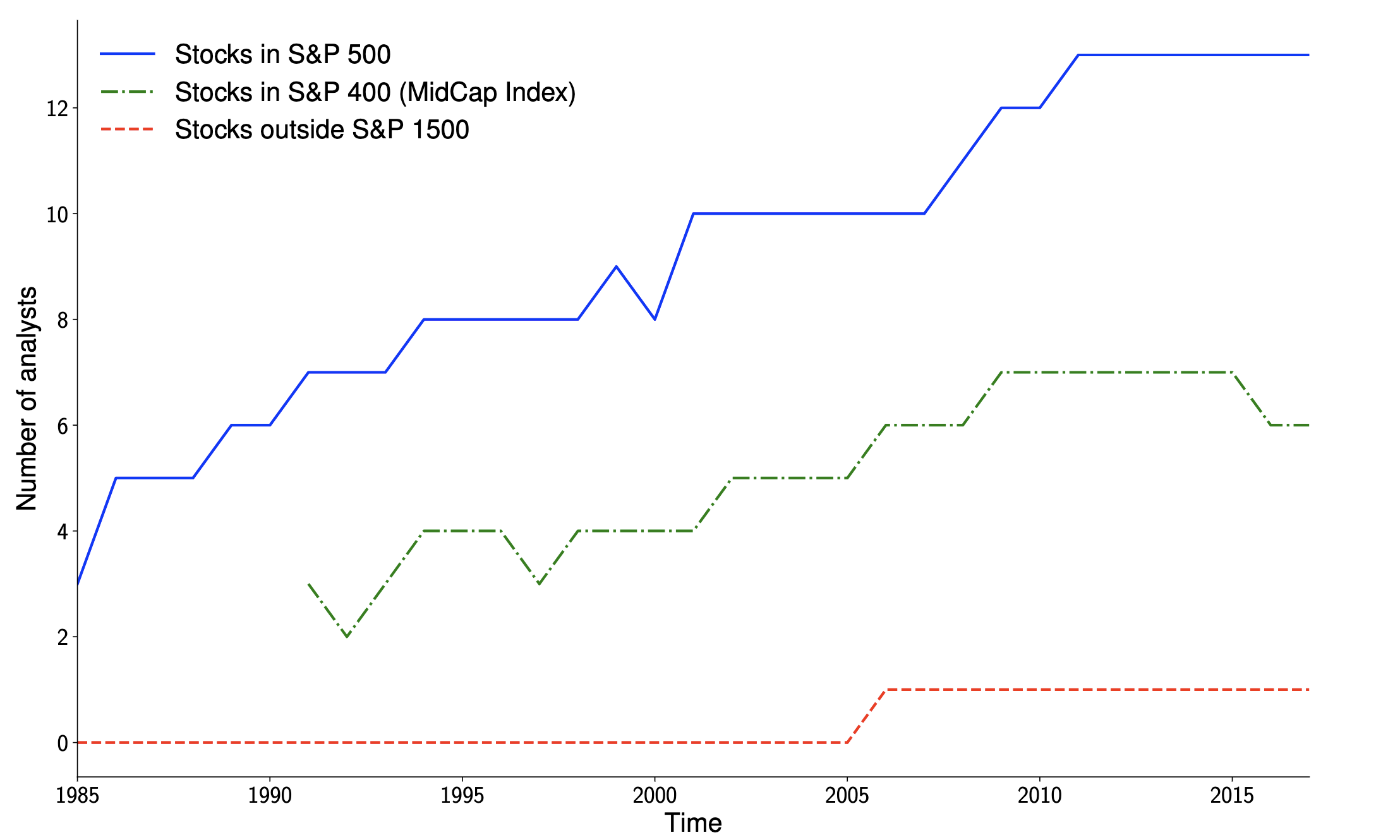
Median coverage in the cross-section of stocks
A closer look at coverage clustering
Conclusions
- Investor attention explains 21.52% of cross-sectional variation in analyst coverage -- second only to firm size.
- For very limited investors attention, analysts are better off sharing a crowded space rather than trying to differentiate and cover neglected stocks.
-
The implications of our model match empirical patterns: the significant analyst coverage clustering in U.S. equities.
- A skewed information supply can disproportionately benefit large firms to the expense of small, "neglected" firms.