Interactions on structured networks
Claudia Merger
supervisors: Prof. Moritz Helias & Prof. Carsten Honerkamp
10.01.2024

Ubiquity of structure

Ubiquity of structure
-
Biological & artificial neural networks
-
Social networks
-
Transportation & infrastructure (trains, power grid, ...)
-
Spin glasses
How can we understand phenomena such as learning, spread of disease, or the emergence of order in these systems?
Ubiquity of structure
Adjacency matrix:
-
Biological & artificial neural networks
-
Social networks
-
Transportation & infrastructure (trains, power grid, ...)
-
Spin glasses
How can we understand phenomena such as learning, spread of disease, or the emergence of order in these systems?
Ubiquity of structure
-
Biological & artificial neural networks
-
Social networks
-
Transportation & infrastructure (trains, power grid, ...)
-
Spin glasses
How can we understand phenomena such as learning, spread of disease, or the emergence of order in these systems?
Adjacency matrix:
Describe interactions on structured systems
Common feature of structured systems: Hubs

degree \(k_i =\) number of connections
hub \( h \): \( k_h \gg \langle k \rangle\)
\( \rightarrow \) degree distribution constitutes a hierarchy on the network
Common feature of structured systems: Hubs
how important are hubs?
Barabási-Albert networks
+
Ising model
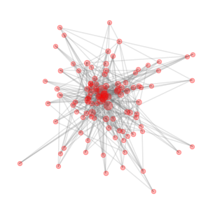
Barabási-Albert networks have hubs
\( N=\) system size,
\( m_0 = 4 \)
Complicated connectivity \( A_{ij} \)
Barabási-Albert networks have hubs
Complicated connectivity \( A_{ij} \)
Ising model defines interactions:
\( N=\) system size,
\( m_0 = 4 \)
Average magnetization
Bianconi et. al., 2001,
Dorogovtsev et. al.,2002
Leone et. al., 2002
Average activity \( m_i = \langle x_i \rangle \)
first order approximation (mean-field theory):
\( m_i=\tanh \bigg( \beta \sum_{j } A_{ij} m_j \bigg) \)
additional assumption: only degree \( k_i \) matters
\(m_i \rightarrow m(k_i) \),
\(A_{ij} \rightarrow p_c(k_i,k_j) \)
same approximation with full connectivity yields wrong results


Bianconi et. al., 2001,
Dorogovtsev et. al.,2002
Leone et. al., 2002
Average magnetization
Bianconi et. al., 2001,
Dorogovtsev et. al.,2002
Leone et. al., 2002
Average activity \( m_i = \langle x_i \rangle \)
first order approximation (mean-field theory):
\( m_i=\tanh \bigg( \beta \sum_{j } A_{ij} m_j \bigg) \)
additional assumption: only degree \( k_i \) matters
\(m_i \rightarrow m(k_i) \),
\(A_{ij} \rightarrow p_c(k_i,k_j) \)
Bianconi et. al., 2001,
Dorogovtsev et. al.,2002
Leone et. al., 2002
Average magnetization

Average activity \( m_i = \langle x_i \rangle \)
first order approximation (mean-field theory):
\( m_i=\tanh \bigg( \beta \sum_{j } A_{ij} m_j \bigg) \)
additional assumption: only degree \( k_i \) matters
\(m_i \rightarrow m(k_i) \),
\(A_{ij} \rightarrow p_c(k_i,k_j) \)
same approximation with full connectivity yields wrong results
Bianconi et. al., 2001,
Dorogovtsev et. al.,2002
Leone et. al., 2002
Beyond the degree resolved picture?
not only degree \( k_i \) matters
but also local connectivity

Fluctuation correction to mean-field model
TAP
mean-field
Thouless, Anderson, Palmer, 1977
Vasiliev &Radzhabov, 1974
Fluctuation correction to mean-field model
TAP
mean-field
Thouless, Anderson, Palmer, 1977
Vasiliev &Radzhabov, 1974

yields an accurate description!
even with the full connectivity
Self-feedback in mean-field equations
mean-field: \( m_i=\tanh \bigg( \beta \sum_{j } A_{ij} m_j \bigg) \)
\( \Rightarrow m_i=\tanh \bigg( \beta \sum_{j } A_{ij} \tanh\left[ \dots + \beta A_{ji} m_i\right]\bigg) \)
Self-feedback in mean-field equations
mean-field: \( m_i=\tanh \bigg( \beta \sum_{j } A_{ij} m_j \bigg) \)
\( \Rightarrow m_i=\tanh \bigg( \beta \sum_{j } A_{ij} \tanh\left[ \dots + \beta A_{ji} m_i\right]\bigg) \)
Self-feedback in mean-field equations
mean-field: \( m_i=\tanh \bigg( \beta \sum_{j } A_{ij} m_j \bigg) \)
\( \Rightarrow m_i=\tanh \bigg( \beta \sum_{j } A_{ij} \tanh\left[ \dots + \beta A_{ji} m_i\right]\bigg) \)
Strongest for hubs!
\( \Rightarrow \) mean-field theory overestimates the importance of hubs
Fluctuation correction to mean-field model
TAP
mean-field
expand \( m_j \) around \( m_i = 0 \)
\( \leftrightarrow \) cavity approach: Mezard, Parisi
and Virasoro, 1986
Thouless, Anderson, Palmer, 1977
\( \Rightarrow \) fluctuations cancel self-feedback

Self-feedback effect, strongest in hubs, is cancelled by fluctuations!
\( \Rightarrow\) description beyond degree resolved
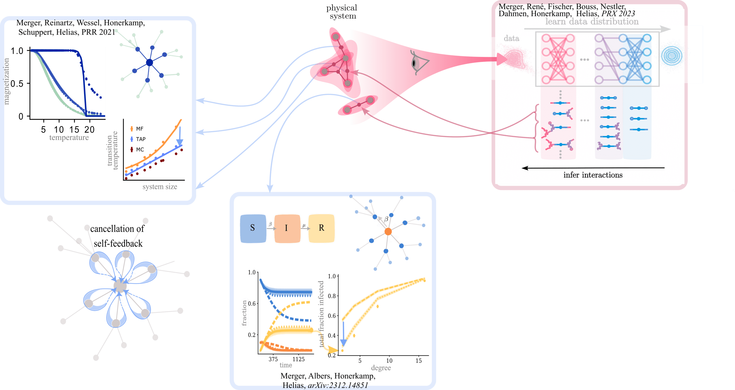
Cancellation of self-feedback
Self-feedback in other systems?
Spread of disease: Models
- Markov process
- Population: Susceptible, Infected, Recovered/Removed

No self-feedback in SIR model

\(t=0\)
\(t=1\)
\(t=2\)
No self-feedback in SIR model
\(t=0\)
\(t=1\)
\(t=2\)
No self-feedback in SIR model
\(t=0\)
\(t=1\)
\(t=2\)
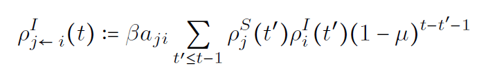
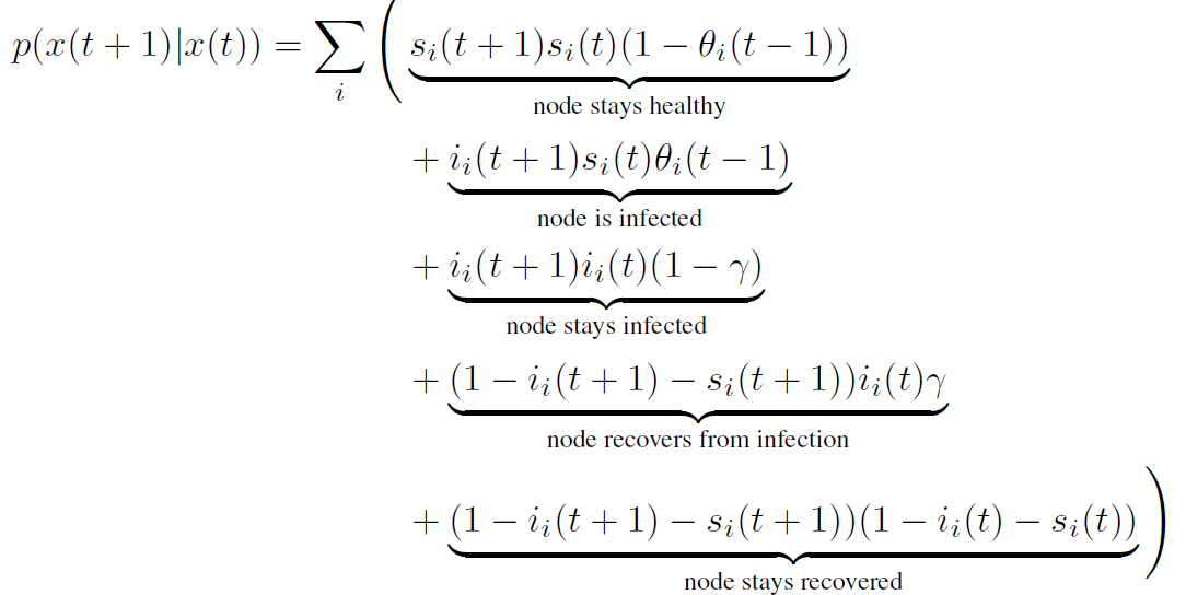
Computing average dynamics
Goal: compute expectation values
\(\rho^{S}_i(t)=\langle S_i(t) \rangle \)
\(\rho^{I}_i(t)=\langle I_i(t) \rangle \)
Notation:
susceptible: \( S_i = 1, I_i =0 \)
infected: \( S_i =0, I_i =1 \)
recovered: \( S_i = I_i =0 \)
Computing average dynamics
Goal: compute expectation values
\(\rho^{S}_i(t)=\langle S_i(t) \rangle \)
\(\rho^{I}_i(t)=\langle I_i(t) \rangle \)
Notation:
susceptible: \( S_i = 1, I_i =0 \)
infected: \( S_i =0, I_i =1 \)
recovered: \( S_i = I_i =0 \)
Computing average dynamics
Goal: compute expectation values
\(\rho^{S}_i(t)=\langle S_i(t) \rangle \)
\(\rho^{I}_i(t)=\langle I_i(t) \rangle \)
Notation:
susceptible: \( S_i = 1, I_i =0 \)
infected: \( S_i =0, I_i =1 \)
recovered: \( S_i = I_i =0 \)
intractable
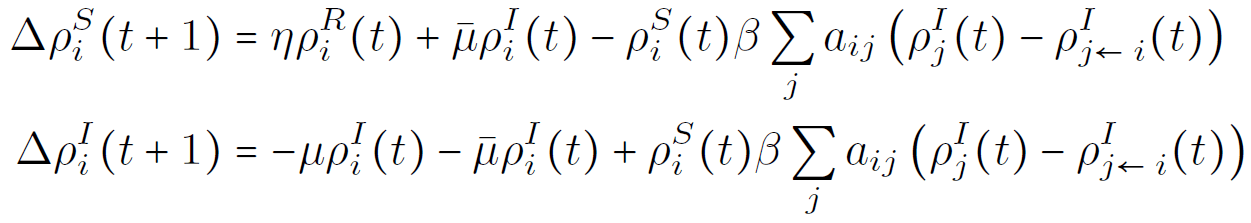
Mean-field equations
approximate agents as independent:
Mean-field equations
approximate agents as independent:
Mean-field equations
approximate agents as independent:
this approximation artificially introduces self-feedback
Self-feedback is a second-order effect
Self-feedback is a second-order effect
- Compute second-order corrections from a systematic expansion(Roudi, Hertz (2011))
- No information about the presence/absence of selffeedback
Self-feedback is a second-order effect
- Compute second-order corrections from a systematic expansion(Roudi, Hertz (2011))
- No information about the presence/absence of selffeedback
1
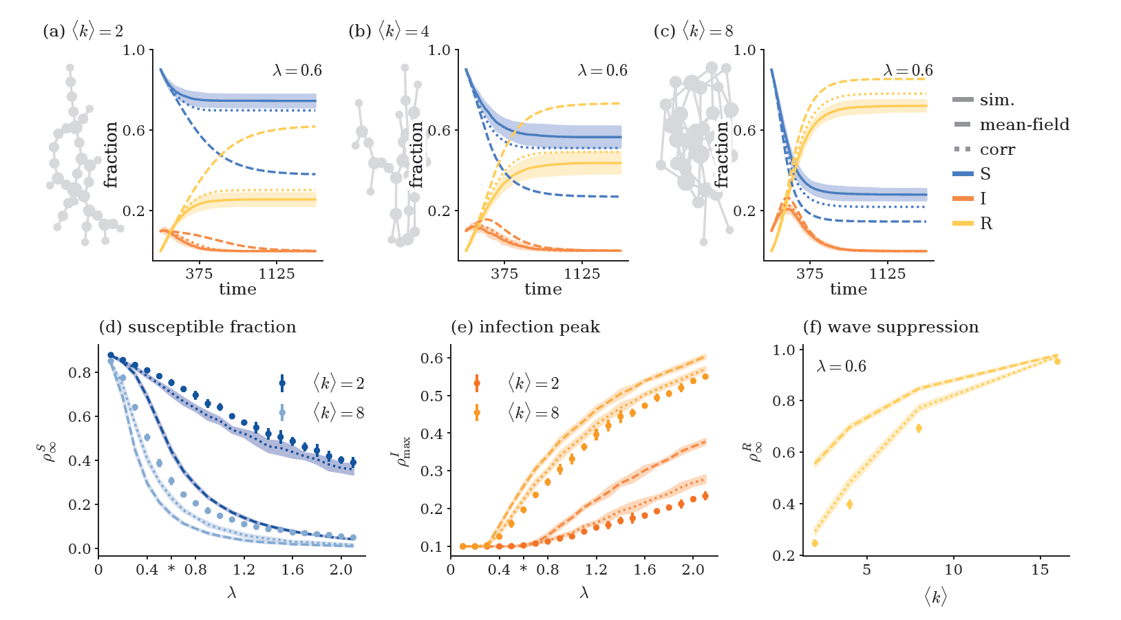
Self-feedback inflates infection curves

Self-feedback inflates infection curves

Self-feedback inflates infection curves
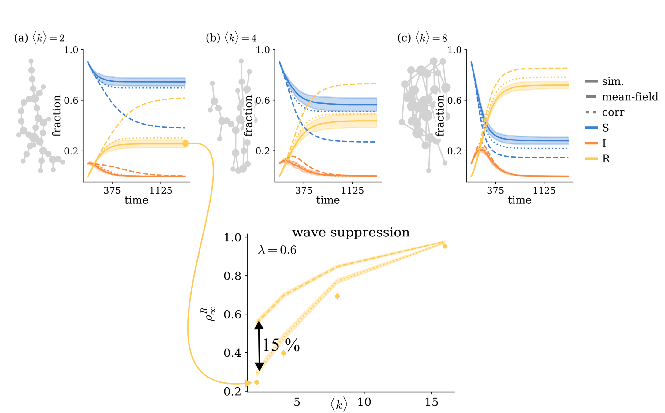
\( \Rightarrow \) Sparsity suppresses activity!
Summary
-
Self-feedback is canceled by fluctuations
- lowering the transition temperature
- reducing the number of infections
- in systems with self-feedback, systematic expansion techniques such as the Plefka expansion can be used
Interactions are effective descriptions of system
Write interacting theory using polynomial action \( S_{\theta} (x) = \ln p_{\theta} (x)\)
\( S_{\theta} (x)= A^{(0)} + A^{(1)}_{i} x_i + A^{(2)}_{ij} x_i x_j +A^{(3)}_{ijk} x_i x_j x_k + \dots \)
Interactions are effective descriptions of system
Write interacting theory using polynomial action \( S_{\theta} (x) = \ln p_{\theta} (x)\)
\( S_{\theta} (x)= A^{(0)} + A^{(1)}_{i} x_i + A^{(2)}_{ij} x_i x_j +A^{(3)}_{ijk} x_i x_j x_k + \dots \)
Example:


Interactions are effective descriptions of system
Write interacting theory using polynomial action \( S_{\theta} (x) = \ln p_{\theta} (x)\)
\( S_{\theta} (x)= A^{(0)} + A^{(1)}_{i} x_i + A^{(2)}_{ij} x_i x_j +A^{(3)}_{ijk} x_i x_j x_k + \dots \)
Example:
how can we find \( S_{\theta} \) given observations of the system?
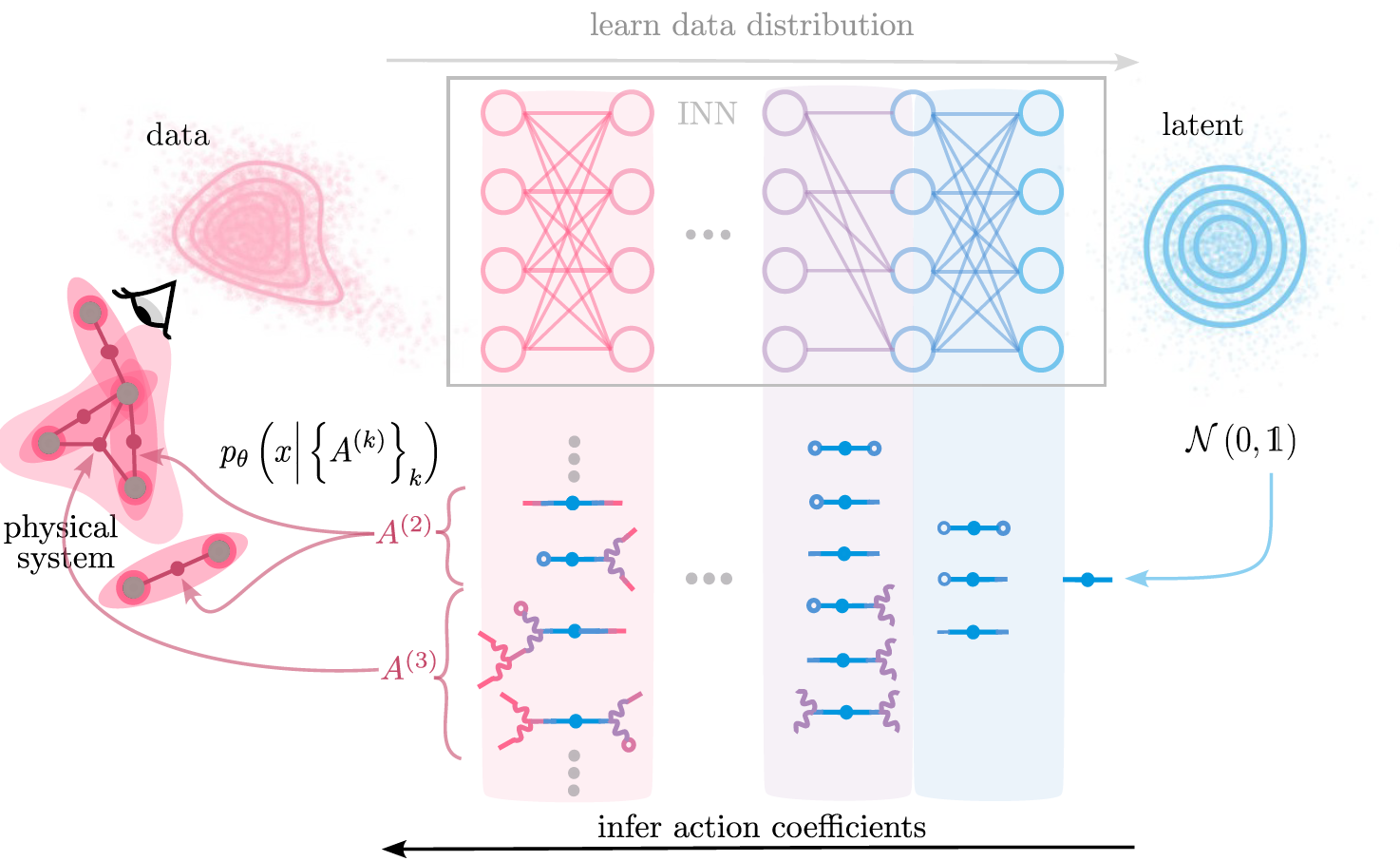
Invertible neural networks learn data distributions
learned data distribution
\( p_{\theta} (x) =p_Z \left( f_{\theta}(x) \right) \big| \det J_{f_{\theta}} (x) \big| \)
loss function
\( \mathcal{L}\left(\mathcal{D}\right) =-\sum_{x \in \mathcal{D}} \ln p_{\theta}(x) \)
NICE (Dinh et. al., 2015 ), RealNVP (Dinh et. al., 2017), GLOW (Kingma et. al. , 2018)
Invertible neural networks learn data distributions
learned data distribution
\( p_{\theta} (x) =p_Z \left( f_{\theta}(x) \right) \big| \det J_{f_{\theta}} (x) \big| \)
loss function
\( \mathcal{L}\left(\mathcal{D}\right) =-\sum_{x \in \mathcal{D}} \ln p_{\theta}(x) \)
generate samples
NICE (Dinh et. al., 2015 ), RealNVP (Dinh et. al., 2017), GLOW (Kingma et. al. , 2018)
Invertible neural networks learn data distributions
take learned data distribution
\( p_{\theta} (x) =p_Z \left( f_{\theta}(x) \right) \big| \det J_{f_{\theta}} (x) \big| \)
write as:
\( S_{\theta} (x)= A^{(0)} + A^{(1)}_{i} x_i + A^{(2)}_{ij} x_i x_j +A^{(3)}_{ijk} x_i x_j x_k + \dots \)
using polynomial \( f_{\theta} \) with \( \det J_{f_{\theta}}(x) = c_{\theta} \)
generate samples
Invertible neural networks learn data distributions
take learned data distribution
\( p_{\theta} (x) =p_Z \left( f_{\theta}(x) \right) \big| \det J_{f_{\theta}} (x) \big| \)
write as:
\( S_{\theta} (x)= A^{(0)} + A^{(1)}_{i} x_i + A^{(2)}_{ij} x_i x_j +A^{(3)}_{ijk} x_i x_j x_k + \dots \)
\(= S_Z \left( f_{\theta}(x) \right) +\ln \big| \det J_{f_{\theta}} (x) \big|\)
using polynomial \( f_{\theta} \) with \( \det J_{f_{\theta}}(x) = c_{\theta} \)
generate samples
Invertible neural networks learn data distributions
starting with \( \ln p_Z( x_L) = S_Z (x_L) = -\frac{x_L^2}{2} +c \)
\( S_{\theta} (x)= S_Z \left( f_{\theta}(x) \right) +\ln \big| \det J_{f_{\theta}} (x) \big|\)
using polynomial \( f_{\theta} \) with \( \det J_{f_{\theta}}(x) = c_{\theta} \)
Mapping of \(x\) \(\rightarrow \) transform of interaction coefficients
\( S_{l-1} \left( x_{l-1} \right) = S_l \left( f_l(x_{l-1}) \right) +\ln | \det J_{f_l} (x)| \)
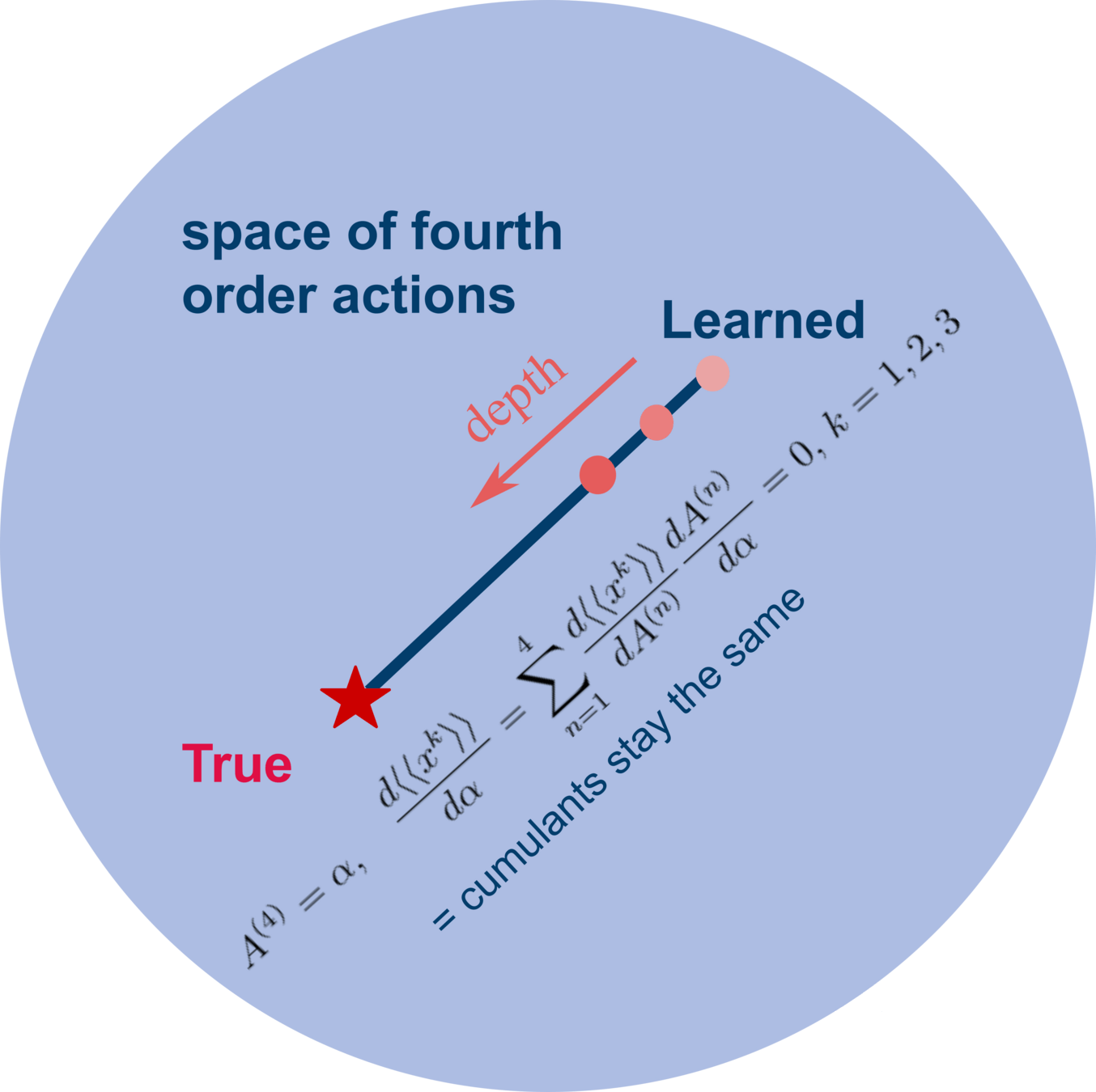
Application: \( \phi^4 \) theory

Application: \( \phi^4 \) theory
- Generate samples from \(p_I(\phi)= e^{S_I(\phi)} \)
- learn new action \(p_{\theta} \) with coefficients \(A^{(k)}\)
- compare \(I^{(k)}\) and \(A^{(k)}\)
Application: \( \phi^4 \) theory
Application: \( \phi^4 \) theory
Application: \( \phi^4 \) theory
depth
depth
Application: \( \phi^4 \) theory

Network reproduces statistics with modified coefficients \( \Rightarrow \) Effective theory
depth
Summary
- learn (effective) higher-order interacting theories from data
- prototype to understand generative learning
Interactions on structured systems
Mapping of \(x\) \(\rightarrow \) transform of interaction coefficients

Layers composed of linear & nonlinear mappings
\(f_l (x_l) =\phi_l \circ L_l \, (x_l) \)
action transform
\( S_{l-1} \left( x_{l-1} \right) = S_l \left( f_l(x_{l-1}) \right) +\ln | \det J_{f_l} (x)| \)
Mapping of \(x\) \(\rightarrow \) transform of interaction coefficients
Layers composed of linear & nonlinear mappings
\(f_l (x_l) =\phi_l \circ L_l \, (x_l) \)
action transform
\( S_{l-1} \left( x_{l-1} \right) = S_l \left( f_l(x_{l-1}) \right) +\ln | \det J_{f_l} (x)| \)
write \( S_l \) as
starting with \( S_Z (z) = -\frac{z_i z_i}{2} +c \)
Mapping of \(x\) \(\rightarrow \) transform of interaction coefficients
Layers composed of linear & nonlinear mappings
\(f_l (x_l) =\phi_l \circ L_l \, (x_l) \)
action transform
\( S_{l-1} \left( x_{l-1} \right) = S_l \left( f_l(x_{l-1}) \right) +\ln | \det J_{f_l} (x)| \)
linear mapping
\( L_l (x_l) = W_l x_l +b_l \)
choose nonlinear mapping
\( \phi_l \) quadratic, invertible with \( \det J_{\phi_l } =1 \)
\( \Rightarrow \, f_l \) quadratic polynomial
Mapping of \(x\) \(\rightarrow \) transform of interaction coefficients
Layers composed of linear & nonlinear mappings
\(f_l (x_l) =\phi_l \circ L_l \, (x_l) \)
action transform
\( S_{l-1} \left( x_{l-1} \right) = S_l \left( f_l(x_{l-1}) \right) +\ln | \det J_{f_l} (x)| \)
linear mapping
\( L_l (x_l) = W_l x_l +b_l \)
choose nonlinear mapping
\( \phi_l \) quadratic, invertible with \( \det J_{\phi_l } =1 \)
\( \Rightarrow \, f_l \) quadratic polynomial with \( \det J_{f_l } = \det W_l \)
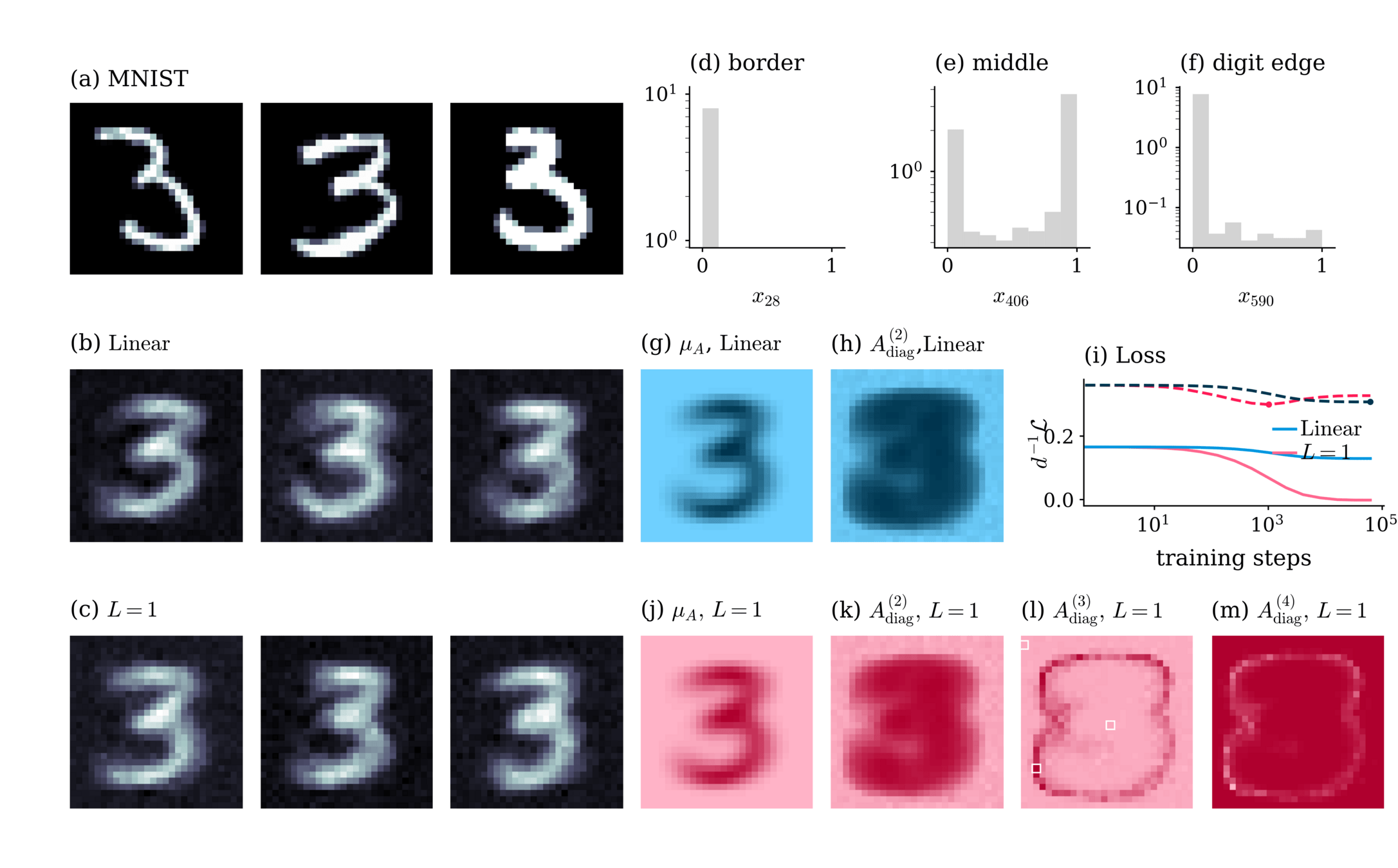
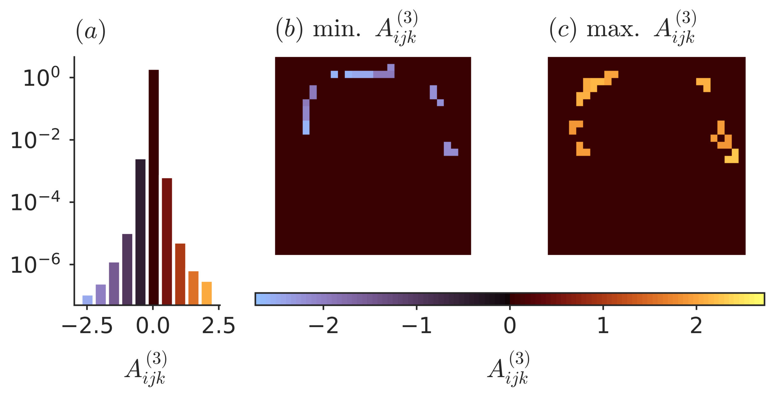
Application: MNIST
\( S_{\theta} (x)= A^{(0)} + A^{(1)}_{i} x_i + A^{(2)}_{ij} x_i x_j +A^{(3)}_{ijk} x_i x_j x_k + \dots \)
Application: MNIST
\( S_{\theta} (x)= A^{(0)} + A^{(1)}_{i} x_i + A^{(2)}_{ij} x_i x_j +A^{(3)}_{ijk} x_i x_j x_k + \dots \)
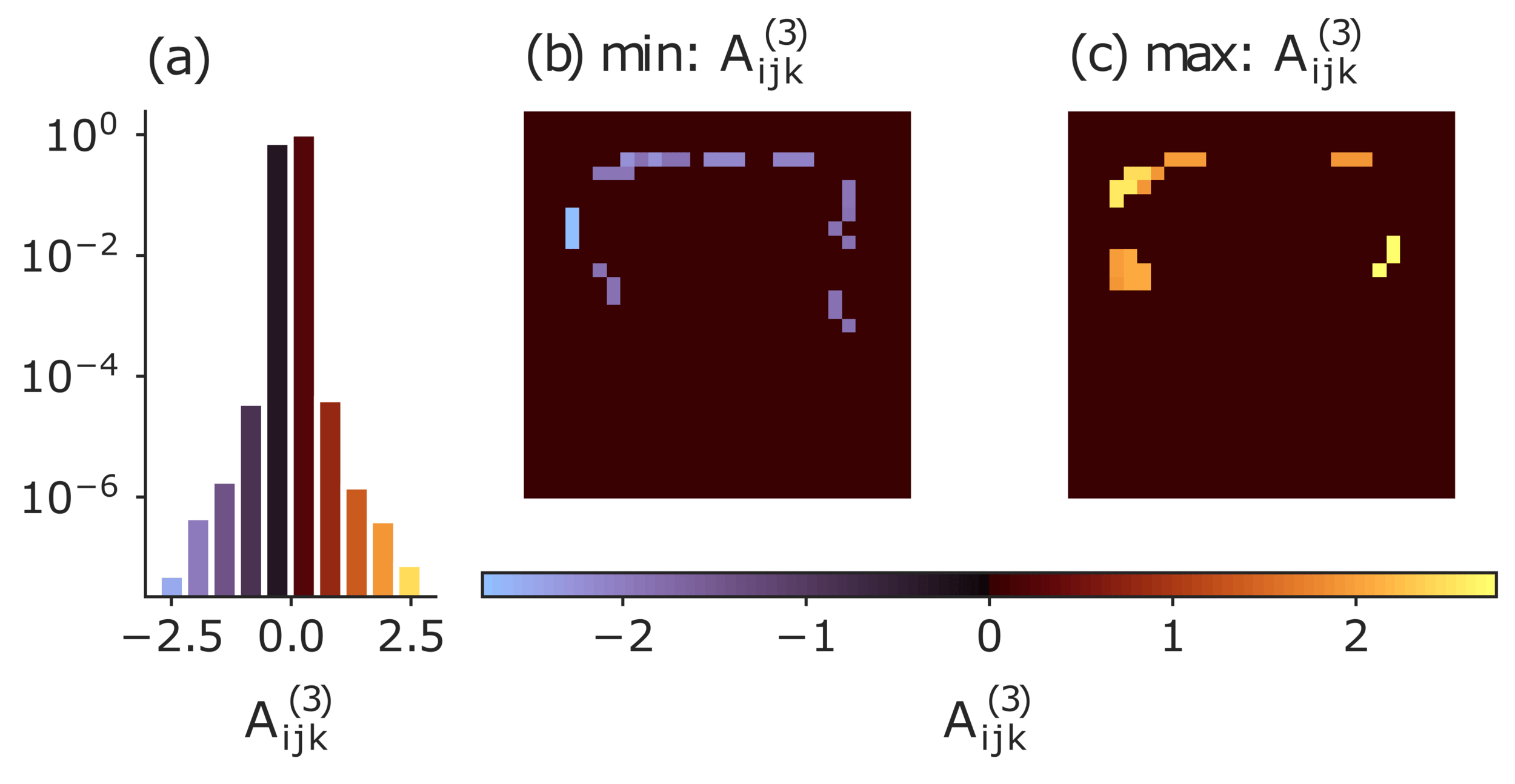
strongest three-point interactions
Application: MNIST
\( S_{\theta} (x)= A^{(0)} + A^{(1)}_{i} x_i + A^{(2)}_{ij} x_i x_j +A^{(3)}_{ijk} x_i x_j x_k + \dots \)

Effective theory
SIR model
\( \Rightarrow \) Sparsity suppresses activity!
Spread of disease: Models
- Markov process
- Population: Susceptible, Infected, Recovered/Removed

SIRS & SIS model
same corrections even though self-feedback is allowed.
only partial cancellation
SIRS & SIS model
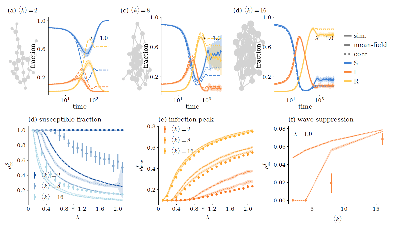
same corrections even though self-feedback is allowed.
only partial cancellation
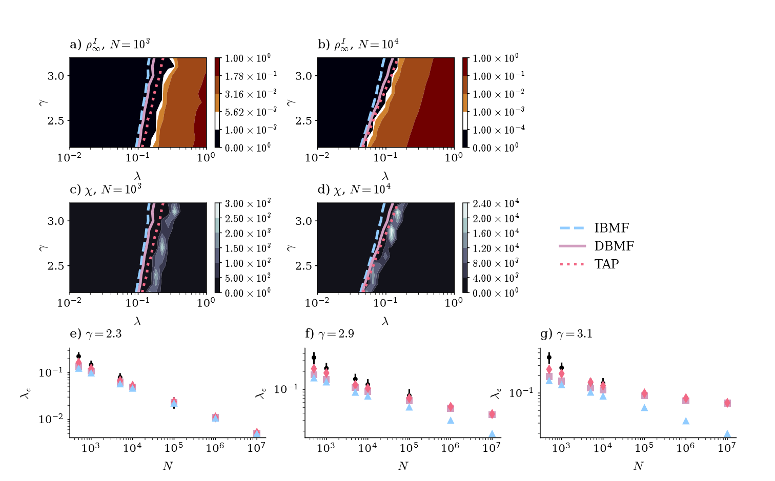
SIRS model
State with finite endemic activity exists,
but at which \( \lambda=\frac{\beta}{\mu} \) ?
SIRS model
State with finite endemic activity exists,
but at which \( \lambda=\frac{\beta}{\mu} \) ?
\( \Rightarrow \) Linearize around \( \rho^I =0\) and check when \(\Delta \rho^I >0 \)
SIRS model
State with finite endemic activity exists,
but at which \( \lambda=\frac{\beta}{\mu} \) ?
\( \Rightarrow \) Linearize around \( \rho^I =0\) and check when \(\Delta \rho^I >0 \)
Mean-field: \(\lambda_c^{-1} = \lambda_a^{max} \)
\(a= \) adjacency matr.
SIRS model
State with finite endemic activity exists,
but at which \( \lambda=\frac{\beta}{\mu} \) ?
\( \Rightarrow \) Linearize around \( \rho^I =0\) and check when \(\Delta \rho^I >0 \)
Mean-field: \(\lambda_c^{-1} = \lambda_a^{max} \)
corrected equation:
\( \lambda_c^{-1} = \lambda_D^{max} \)
\(a= \) adjacency matr.
Mean-field: \(\lambda_c^{-1} = \lambda_a^{max} \)
corrected equation:
\( \lambda_c^{-1} = \lambda_D^{max} \)
Mean-field: \(\lambda_c^{-1} = \lambda_a^{max} \)
corrected equation:
\( \lambda_c^{-1} = \lambda_D^{max} \)
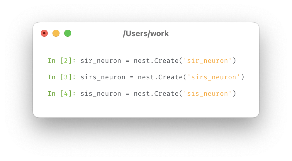
Simulation with NEST
Difficulty: Spiking neurons \( \rightarrow \) neurons with 3 discrete states
basis for implementation: binary neurons
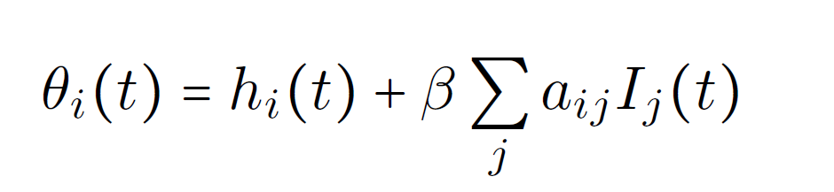
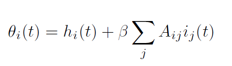
idea: communicate changes to \( \theta_i \)
signal change of state via spikes:
Spike with multiplicity 1: \( S \rightarrow I \)
Spike with multiplicity 2: \( I \rightarrow S,R \)
Simulation with NEST
Monte-Carlo
"Ground truth"
"conventional" Metropolis Monte Carlo: Hubs freeze out
Parallel Tempering
Swedensen and Wang,1986
\( T \)
\(\beta_i \)
\(\beta_j \)
\( p_{ij} = \min \left( 1, e^{(E_i-E_j)(\beta_i -\beta_j)}\right) \)
Timo Reinartz, Stefan Wessel
Beyond the degree resolved picture?
not only degree \( k_i \) matters
but also local connectivity
first order approximation (mean-field theory):
\( m_i=\tanh \bigg( \beta \sum_{j } A_{ij} m_j \bigg) \)
\( \rightarrow \) yields incorrect results!

Beyond the degree resolved picture?
not only degree \( k_i \) matters
but also local connectivity

first order approximation (mean-field theory):
\( m_i=\tanh \bigg( \beta \sum_{j } A_{ij} m_j \bigg) \)
\( \rightarrow \) yields incorrect results!
Fluctuation correction to mean-field model
TAP
mean-field
Thouless, Anderson, Palmer, 1977
Vasiliev &Radzhabov, 1974
yields a more accurate description!
even with the full connectivity

SIR model
Analogous 2-state problem:
Roudi, Y. & Hertz, J. Dynamical TAP equations for non-equilibrium Ising spin glasses. Journal of Statistical Mechanics: Theory and Experiment 2011, P03031 (2011).
update probability:
Compute second order corrections!
Analogous 2-state problem:
Roudi, Y. & Hertz, J. Dynamical TAP equations for non-equilibrium Ising spin glasses. Journal of Statistical Mechanics: Theory and Experiment 2011, P03031 (2011).
update probability:
Compute second order corrections!
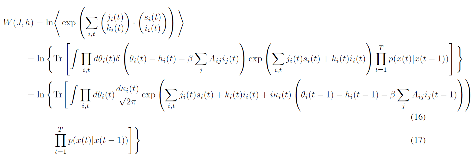
Cumulant generating functon
Compute second order corrections!
Cumulant generating functon
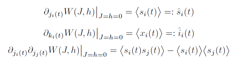
Compute second order corrections!
Cumulant generating functon
Compute second order corrections!
Cumulant generating functon
Compute second order corrections!
Cumulant generating functon
Effective action: Legendre transform

Effective action: Legendre transform
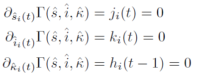
eq. of state
Effective action: Legendre transform
eq. of state
mean-field
flu. correction / "TAP term"
Plefka expansion: Expansion in \( \beta \)