Active Tactile Pose and Shape Estimation of Highly Dynamic Objects
Ethan K. Gordon, Bruke Baraki, Hien Bui, Michael Posa
Supported By: NSF CAREER (FRR-2238480) and the RAI Institute
ethan@ethankgordon.com
COMPUTING INFORMATION THROUGH DYNAMICS
- Learning Difficulty: gradients of dynamics \(f\) are near-0 or near-\(\infty\), which is not amenable to learning.
- Solution: add inner optimization over contact forces \(\lambda\). Trade-off: solving a (fast) QP each gradient step for better gradients.
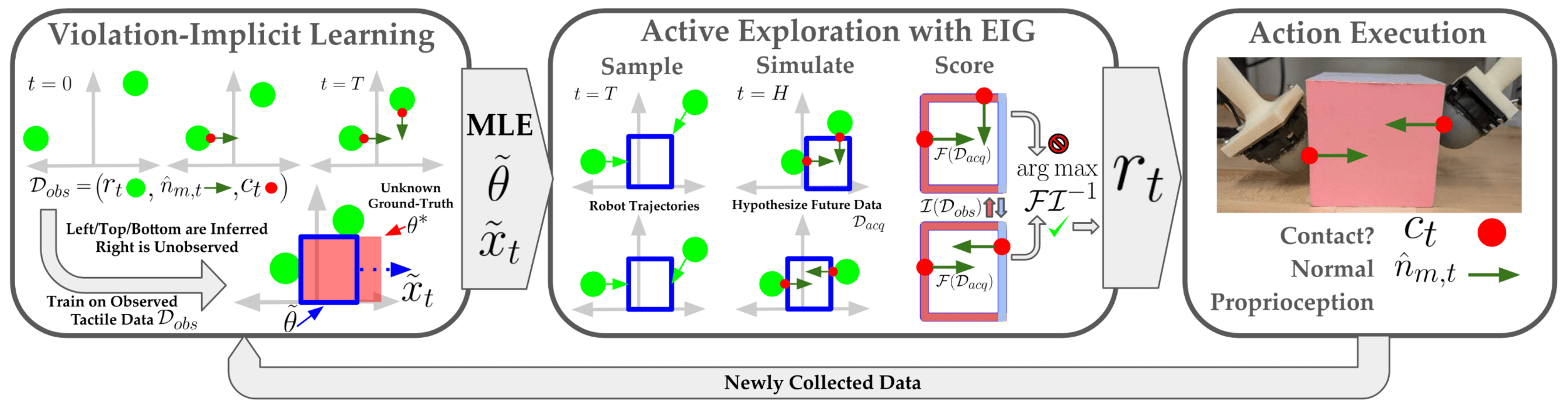
\(\mathcal{L} = -\log p(m_t | \theta, x_{<T}) =\sum_t -\log p(m_t | \theta, x_t) + ||x_t - f_\theta(x_{t-1}, \lambda)||^2\)
Where \(\lambda = \min g_\theta(x, \lambda)\)
\(\mathcal{L} = \sum_t \min_\lambda -\log p(m_t | \theta, x_t) + ||x_t - f_\theta(x_{t-1})||^2 + g_\theta(x, \lambda)\)
Physics Constrained MLE with Trajectory Optimization
Violation-Implicit (VIMP) Loss
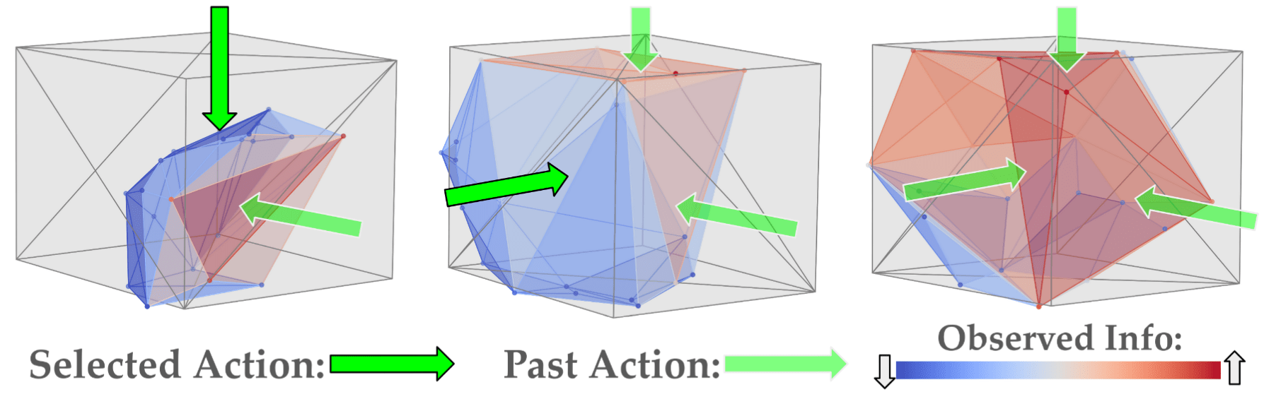
- Observed Info: empirical variance of log-likelihood grad
\(\mathcal{I} = \sum_{m_t} \left(\nabla_{\theta, x_T}\log p(m_t|\theta, x_T)\right)^2\)
- Fisher Info: expected variance given future measurements
\(\mathcal{F} = \mathbb{E}_{m_t}\left[\mathcal{I}(m_t, \theta, x_{H>T})\right]\)
- Sample future actions, Simulate to estimate \(\mathcal{F}\), then maximize Expected Information Gain (EIG)
\(EIG := \log\det\left(\mathcal{F}\mathcal{I}^{-1} + \mathbf{I}\right)\)
w.r.t. Current Time T
w.r.t. Future Time H
Challenge: How to compute \(\nabla \log p(m_t | x_T)\), i.e. sensitivity of past measurements to the future state?
Computing \(g=\nabla \log p(m_t | x_T)\)
Rejected: Backwards Simulation
\(g = \nabla \log p(m_t|x_t(x_T))\)
Ill-defined for frictional contact.
Baseline 1: Identity Jacobian
\(\nabla_{x_T}x_t = \nabla_{x_t}x_T = \mathbb{I}\)
Treats object as quasi-static
Baseline 2: Diffsim
Compute \(g=\nabla \log p (m_t|x_0)\) instead.
Poorly conditioned numerically
Proposed: Marginalize + Sample
\(g \approx \nabla \log \sum_{x_t}p(m_t|x_t)p(x_t|x_T)\)
Sample \(x_t\) w/ MCMC, use vimp loss \(\mathcal{L}\)
\(\approx softmax_{x_t}(\log p(m_t|x_t)) \cdot \nabla\mathcal{L}\)
EXPERIMENT SETUP
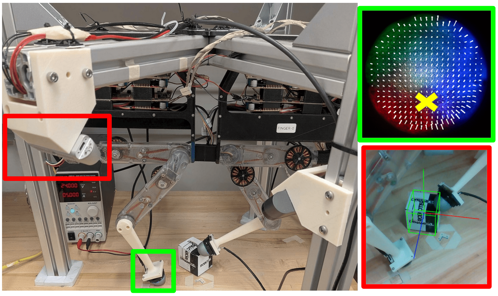
Hardware Setup
- Modified Trifinger Robot
- Densetact 2.0 (Do, 2023)
- Contact Boolean \(c_t\) and Normal \(\hat{n}_t\) computed with Optical Flow and a Helmholz-Hodge Decomposition
- FoundationPose for Ground-Truth only
Experiment Design
- Action: 1s motion towards estimated object centroid
- Random Baseline: Randomize approach direction
- EIG (Ours): Choose the approach to maximize EIG, sampling-based optimization with Gaussian Cross-Entropy Method
Project Website
BASELINE RESULTS AND CONCLUSION

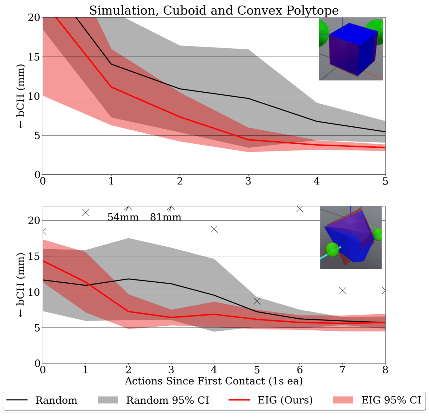
- Simulated results for cuboid and polytope parameterizations.
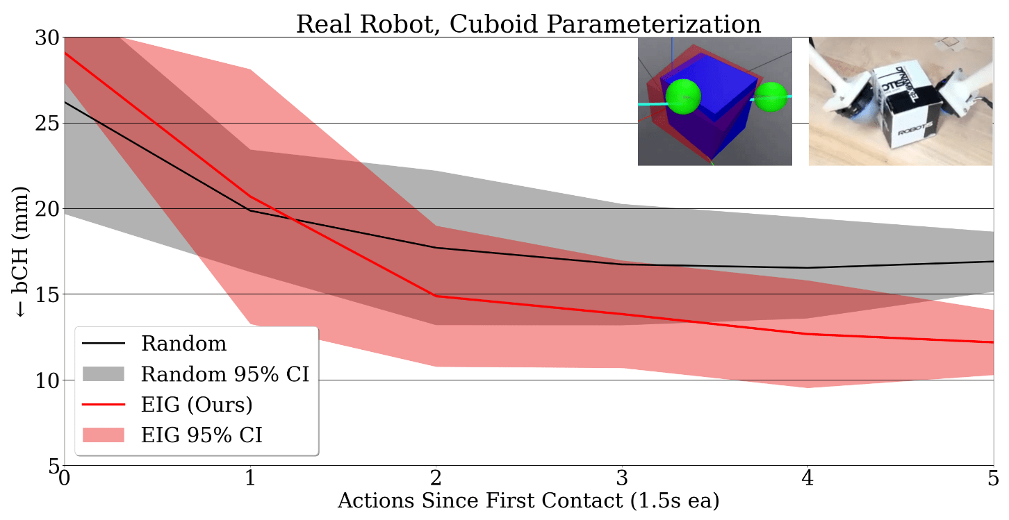
- Real robot results on cuboid
- Example learning curves. Observed information increases with more data.
- Bidirectional Chamfer Distance (bCH) Evaluation Metric
- Identity Jacobian EIG showed significant improvement over object-directed actions from random approach directions.
Next Steps: expand experiment to proposed (marginalize + sample) EIG formulation.
INTRODUCTION
- Learning a physical model online can improve data efficiency, predictability, and reuse between tasks.
- Previous Tactile System Identification Work: Static Objects and/or Strong Shape Priors and/or 2D
- Learning: apply ContactNets-style violation-implicit learning (Pfommer, CoRL 2020) to pose estimation, avoiding the numerical stiffness inherent in rigid-body contact dynamics.
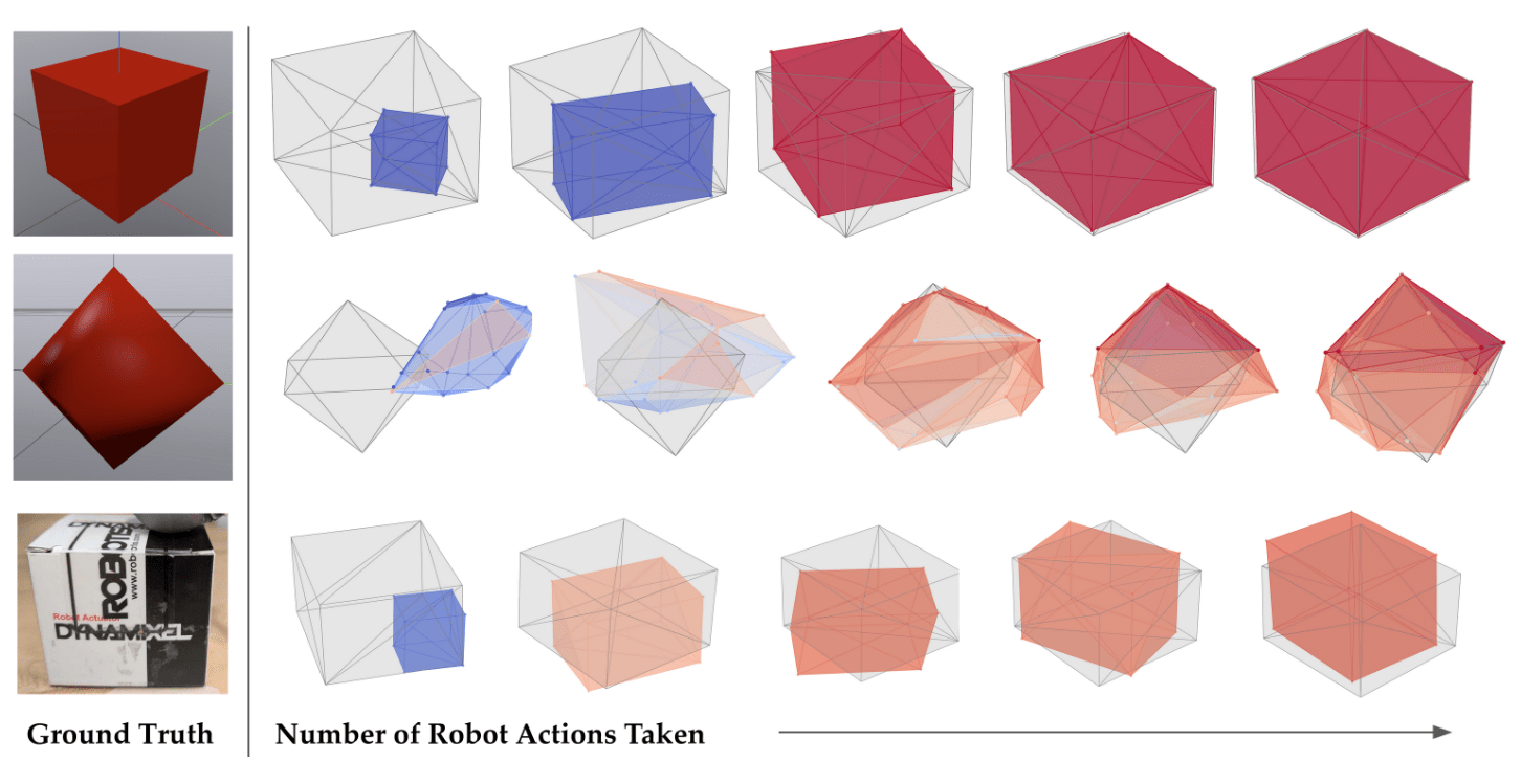
- We learn cuboid and convex polyhedra with less than 10s of randomly collected data.
- Exploration: maximizing Expected Info Gain (EIG) leads to significantly faster learning.
Challenge: Use only tactile data to find the pose and geometry of an arbitrary dynamic convex object.
Fast sampling with learned trajectory
Active Tactile Pose and Shape Estimation of Highly Dynamic Objects
Ethan K. Gordon, Bruke Baraki, Hien Bui, Michael Posa
Supported By: NSF CAREER (FRR-2238480) and the RAI Institute
ethan@ethankgordon.com
METHOD OVERVIEW
- Learning Difficulty: gradients of dynamics \(f\) are near-0 or near-\(\infty\), which is not amenable to learning.
- Solution: add inner optimization over contact forces \(\lambda\). Trade-off: solving a (fast) QP each gradient step for better gradients.
\(-\log p(m_t | \theta, x_{<T}) =\sum_t -\log p(m_t | \theta, x_t) + ||x_t - f_\theta(x_{t-1}, \lambda)||^2\) s.t. \(\lambda = \min g_\theta(x, \lambda)\)
\(\mathcal{L} = \sum_t \min_\lambda -\log p(m_t | \theta, x_t) + ||x_t - f_\theta(x_{t-1})||^2 + g_\theta(x, \lambda)\)
Physics Constrained MLE with Trajectory Optimization
Violation-Implicit (VIMP) Loss
- Observed Info: empirical variance of log-likelihood grad
\(\mathcal{I} = \sum_{m_t} \left(\nabla_{\theta, x_T}\log p(m_t|\theta, x_T)\right)^2\)
- Fisher Info: expected variance given future measurements
\(\mathcal{F} = \mathbb{E}_{m_t}\left[\mathcal{I}(m_t, \theta, x_{H>T})\right]\)
- Sample future actions, Simulate to estimate \(\mathcal{F}\), then maximize Expected Information Gain (EIG)
\(EIG := \log\det\left(\mathcal{F}\mathcal{I}^{-1} + \mathbf{I}\right)\)
w.r.t. Current Time T
w.r.t. Future Time H
Challenge: How to compute \(g=\nabla \log p(m_t | x_T)\), i.e. sensitivity of past measurements to the future state?
Rejected: Backwards Simulation
\(g=\nabla \log p(m_t|x_t(x_T))\)
Ill-defined for frictional contact.
Baseline 1: Identity Jacobian \(\nabla_{x_T}x_t = \nabla_{x_t}x_T = \mathbb{I}\)
Treats object as quasi-static
Fails for left example: \(\mathcal{F}\) only non-0 for 1 face.
Baseline 2: Differentiable Simulation
Compute \(g=\nabla \log p (m_t|x_0)\) instead.
Poorly conditioned numerically
Same as learning difficulty (above).
Proposed: Marginalize + Sample
\(g \approx \nabla \log \sum_{x_t}p(m_t|x_t)p(x_t|x_T)\)
\(\approx softmax_{x_t}(\log p(m_t|x_t)) \cdot \nabla\mathcal{L}\)
Sample \(x_t\) w/ MCMC, use vimp loss \(\mathcal{L}\)
COMPUTING INFORMATION THROUGH DYNAMICS
- Trifinger with Densetact 2.0 (Do, 2023)
- Contact Boolean \(c_t\) and Normal \(\hat{n}_t\) computed with Optical Flow and a Helmholz-Hodge Decomposition
- FoundationPose for Ground-Truth only
Project Website
BASELINE EXPERIMENT AND CONCLUSION
- (Left): Simulated (top) and real (bottom) results for cuboid and polytope parameterizations.
- Identity Jacobian EIG showed significant improvement over object-directed actions from random approach directions.
Next Steps: expand experiment to proposed (marginalize + sample) EIG formulation.
INTRODUCTION
- Learning a model online can improve data efficiency, predictability, and reuse between tasks.
- Previous Tactile System Identification Work: Static Objects and/or Strong Shape Priors and/or 2D
- Learning: apply ContactNets-style violation-implicit learning (Pfommer, CoRL 2020) to pose estimation, avoiding the numerical stiffness inherent in rigid-body contact dynamics.
- We learn cuboid and convex polyhedra with less than 10s of randomly collected data.
- Exploration: maximizing Expected Info Gain (EIG) leads to significantly faster learning.
Challenge: Use only tactile data to find the pose and geometry of an arbitrary dynamic convex object.
Fast sampling with learned trajectory
Example (right): We have only touched 1 face, but the dynamics provides info about 3 faces.
\(m_1\)
\(x_1\)
\(m_T\)
\(x_T\)
\(m_1\)
\(x_1\)
\(m_2\)
\(x_2\)