Active Tactile Exploration
for Rigid Body State Estimation
Ethan K. Gordon, Bruke Baraki, Michael Posa


<Items in Brackets are Meta Notes / Still in Progress. Feedback Appreciated!>
Known / Estimated:
-
Object Geometry
-
Object Pose
- Object Mass / Inertia
- Frictional Properties
IN Robotics, Models are Powerful
Max Planck Real Robotics Challenge 2020
Arbitrary Convex Object Repose Task
Bauer et al. "Real Robot Challenge: A Robotics Competition in the Cloud". NeurIPS 2021 Competition.
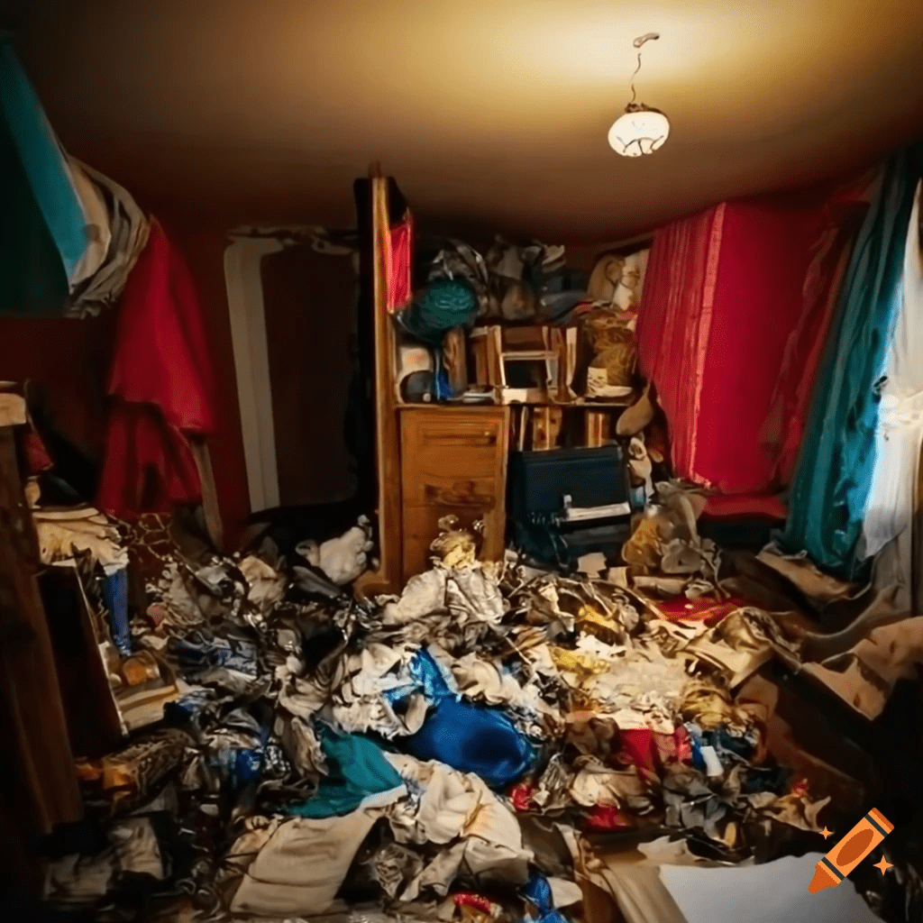
Models are difficult to build Online
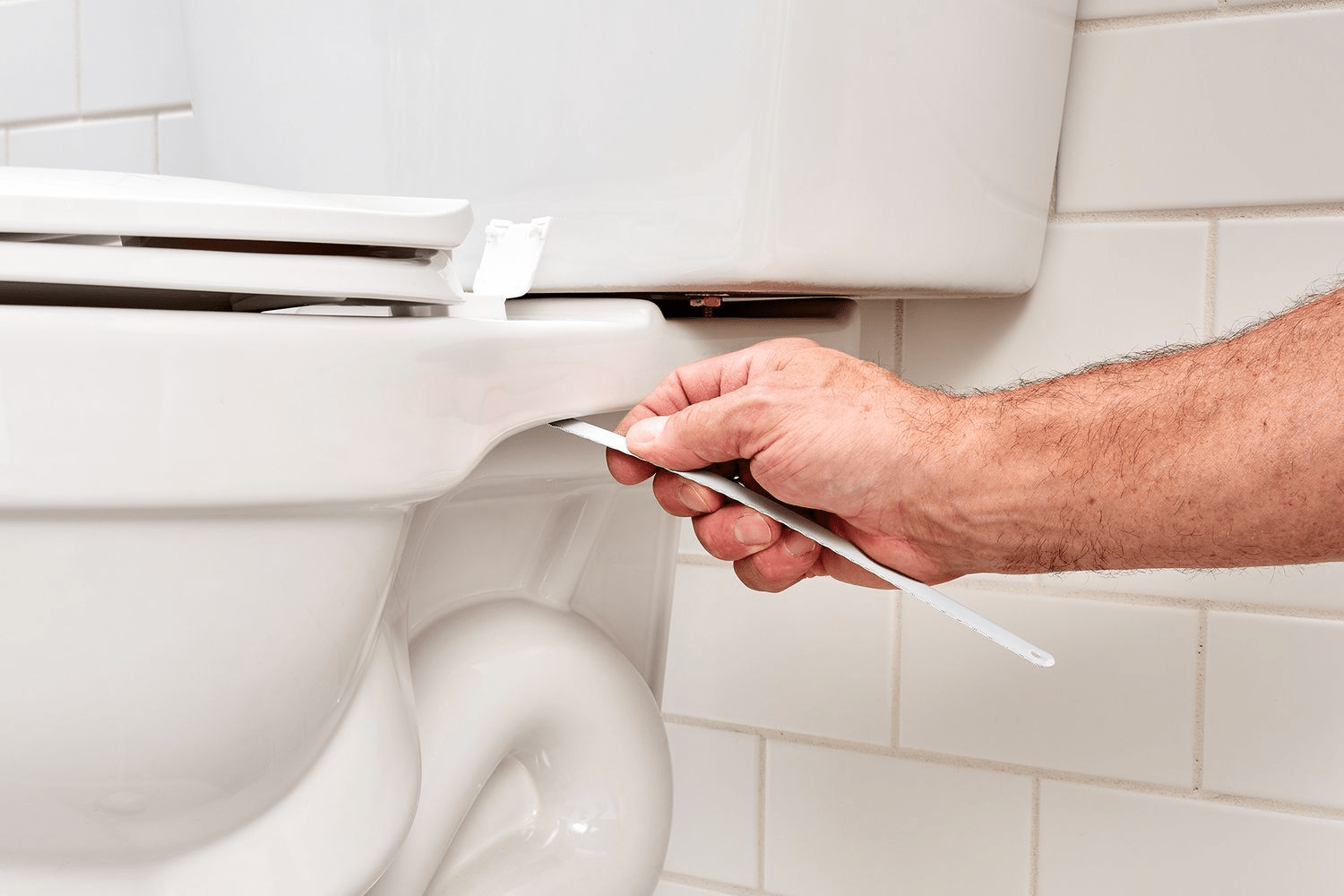
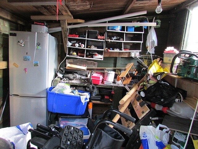
-
Occlusions / Darkness
-
Clutter
-
Heterogeneous Materials
- Broken Objects
Visual Model Learning
Structure from Motion (SFM)
Bianco et al. "Evaluating the Performance of Structure from Motion Pipelines", Journal of Imaging 2018
Wen et al. "BundleSDF: Neural 6-DoF Tracking and 3D Reconstruction of Unknown Objects", CVPR 2023
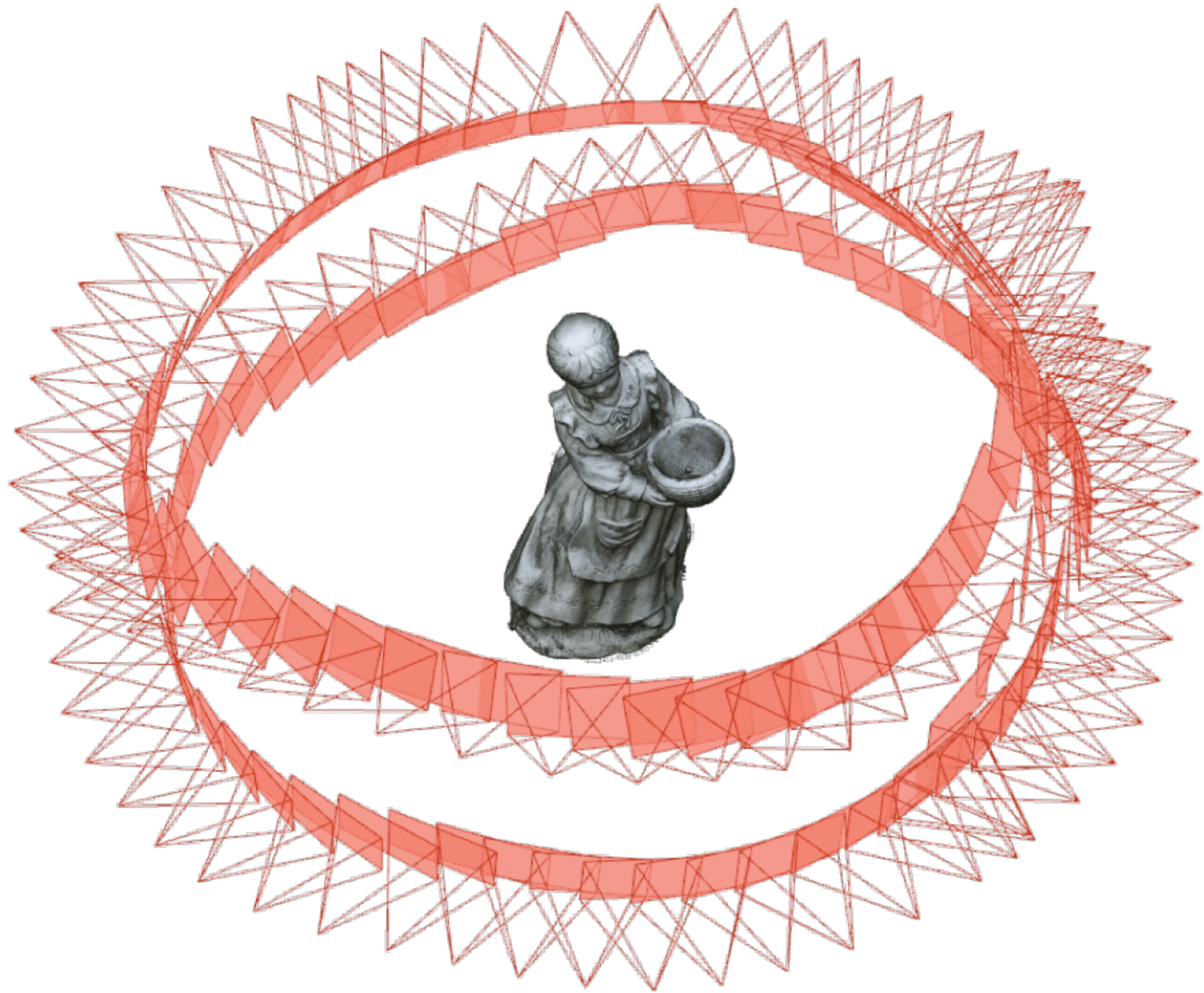
Geometry from Video
Pros: Spatially Dense, Mature HW and SW
Cons:
- Occlusions / Darkness
- SFM: can't capture physical properties
- Video: What's doing the manipulating?
State of the art Tactile Model Learning
Hu et al. "Active shape reconstruction using a novel visuotactile palm sensor", Biomimetic Intelligence and Robotics 2024
Xu et al. "TANDEM3D: Active Tactile Exploration for 3D Object Recognition", ICRA 2023
Single-Finger Poking: No friction or inertia.
Utilizes discrete object priors.
Spatially Sparse Data -> Active Learning
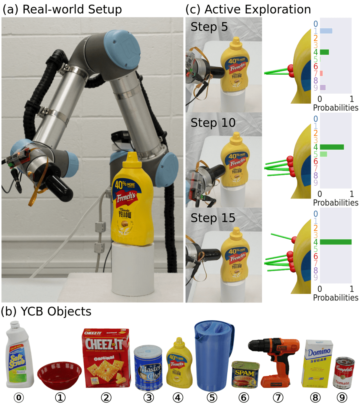
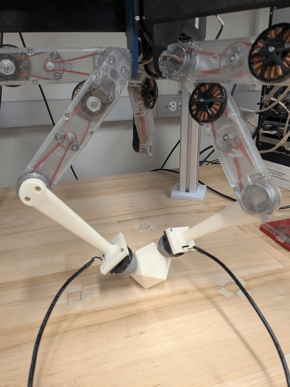
Active Tactile Exploration: Problem Statement

?
Assumptions:
-
Rigidity
-
Convexity
- Coulomb friction
What we know / measure:
-
Robot state trajectory \(r[t]\)
-
Contact force \(\lambda_m[t]\)
- Contact normal \(\hat{n}_m[t]\)
Unknown object properties:
-
State \(x[t]\)
-
Geometry \(\theta\)
- Inertial properties \(\theta\)
- Frictional properties \(\theta\)
Measurement Probability Model
<Gaussian: Major (likely incorrect) Assumption>
<A Gamma is likely more accurate (>0 and mean-dependent variance, with variance -> 0 when mean -> 0). However, in practice, a Gaussian estimator often achieves similar performance to a Gamma.>
Minimize as a loss function for a Maximum Likelihood Estimate
Given a simulator that can compute \(\hat{\lambda}\)
ONe Possibility is Differential Simulation + Shooting
Anitescu. "Optimization-based simulation of nonsmooth rigid multibody dynamics,” Mathematical Programming 2006
Improving Stability with an Implicit Loss
Bianchini et al. "Generalization Bounded Implicit Learning of Nearly Discontinuous Functions,” L4DC 2022
<TODO: Replace with self-made plot>
DiffSim + Shooting Limitations:
- Sensitivity to x[0]
- Discontinuities given process noise \(\epsilon_p\)
- Only gets worse with smaller dt
Solution is to bring the optimization into the loss function.
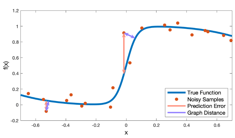
MSE -> Graph Distance
Violation Implicit Loss summary
Pfommer et al. "ContactNets: Learning Discontinuous Contact Dynamics with Smooth, Implicit Representations,” CoRL 2020
Complementarity:
Penetration:
Measurement:
Prediction:
Power Dissipation:
(Relaxed in Anitescu)
Learning <Preliminary> Results
Real Time Simulated Data Collection, Real Time Gradient Descent
active exploration: What is Information?
We want to (possibly) be surprised
\(\Theta\)
\(\mathcal{L}\)
Ideally information is local
(i.e. no belief distribution on \(\Theta\))
\(\Theta\)
\(\mathcal{L}\)
\(\Theta\)
\(\mathcal{L}\)
\(\Theta\)
\(\mathcal{L}\)
- Estimate \(\hat{\Theta}\)
- Choose \(r\)
- Observe (random) \(\lambda_m\)
\(\hat{\Theta}\)
\(r\)
Fisher Information: Variance of the score
"log-likelihood"
"score"
We are surprised if, at \(\hat{\Theta}\), the score varies a lot with new data.
"Fisher Information"
Fisher Information definitions
\(\hat{\Theta}\) is a Maximum Likelihood Estimate
(outer product)
The variance of the gradient is the expected sensitivity of the gradient to small changes in the loss function.
\(\Theta\)
\(\mathcal{L}\)
Fisher Information definitions
The variance of the gradient is the expected sensitivity of the gradient to small changes in the loss function.
\(\Theta\)
\(\mathcal{L}\)
Mathematically requires "certain regularity conditions":
- \(\mathbb{E}\) is necessary: requires swapping integral and derivative order
- Requires the \(\log\mathbb{P}\): uses normalization of the probability distribution
How to calculate Fisher Information
-
Start with the probability model: \(\lambda_m = \hat{\lambda} + \epsilon\)
- Not Necessarily Gaussian
- For a given \(r\), simulate forward to find \(\hat{\lambda}\)
- Sample possible forward values for \(\lambda_m\)
- Autodiff calculate \(\nabla_\Theta\mathcal{L}\Bigr\rvert_{\hat{\Theta}}\) for each sample
- Take the empirical mean of the outer products
<What is the right probability model? Can also simulate with process noise>
<Currently I have a bug in my implementation, so I don't have complete results.
I feed in \(\lambda_m\) as post-optimization impulses. Instead I need to re-optimize in calculation of \(\mathcal{L}\)>
Example: Complementarity
Example with action library
\(tr(\mathcal{I})\) = [1388150.4359, 2878543.4818, 2905122.0841]
For Actions: [2-finger X Pinch, 2-finger Z Pinch w/ Ground, 1-finger Cube Corner Hit]
Expected Info Gain: avoid redundancy
- \(\mathcal{I}\) is independent of past data \(\mathcal{D}\)
- Same action will be taken every time!
- Solution: de-prioritize info we've already seen.
Note \(\sum_\mathcal{D}\left(\nabla_\Theta\mathcal{L}\Bigr\rvert_{\hat{\Theta}}\right) = \nabla_\Theta\left(\sum_\mathcal{D}\mathcal{L}\Bigr\rvert_{\hat{\Theta}}\right) = 0\), since \(\hat{\Theta}\) is the MLE
Final MAximization Problem
Choosing a scalarization is a whole field of study. Common choices include:
- A (average): \(tr(EIG)\) -> average EIG across parameters
- E (eigenvalue): \(\min(eigenvalue(EIG))\) -> prioritize parameter we know the least about.
- D (determinant): \(det(EIG)\) -> maximize area of the "uncertainty ellipse" around the score.
Thank You!

<Other Funding Orgs>