Intro to networks
Part I
Open up graphcommons.com
You can sign in however you want, just remember what you used!

BUT SKIP THE TUTORIAL


We're going to import a csv. Download this one, then upload it using "Import edges"
Ignore "Import nodes" for now and hit Continue
Your import should look like this, then Save
It may take a while to process, so be patient!

What a mess!
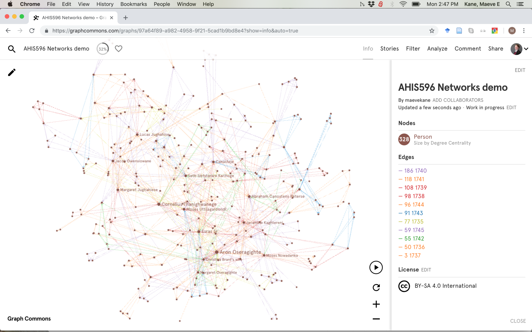
Each dot is a person, or a "node." The lines that connect them are "edges." We're looking at all connections within a church congregation from 1735-1745 (Your numbers may be larger than in the examples, I gave you a different slice of the congregation)
Hovering over the play button gives you some layout options like show/hide labels. Force Atlas and Force Directed tells the computer how close or far to place each node from each other. Try playing around--if you hit play, the layout will change based on your settings..

Filters work just like spreadsheets and other programs. Let's add a filter.

For now, we'll only filter our edges (the connections between each person)
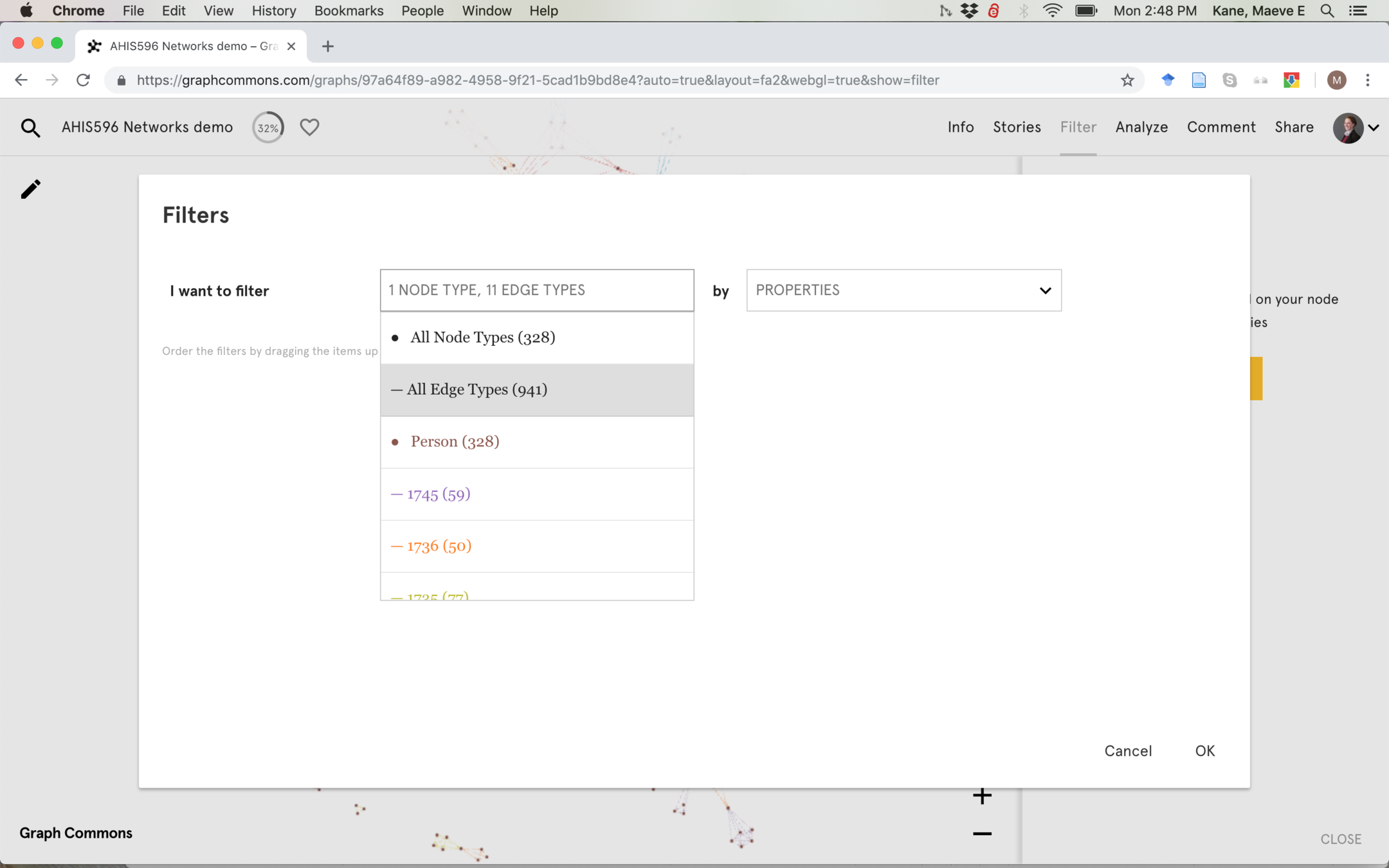
GraphCommons isn't quite smart enough to order our years correctly, but our filter lets us select which years to display.

By turning off all years except for 1735, we can start to see how the network evolved.

How does the network change over time as you add more years? Who are the major connectors who bring small sub-networks into connection? Hover over the nodes to see more about them.

Optional: To customize the look of your network, click "Carto"

Using a color tool like Chroma.js, find a sequential series of colors and get their hex keys.

You can enter these hex keys for each year in Carto

You can also color the nodes and resize them.

By default, the nodes are sized by their degree centrality, or the number of connections they have to others. In degree is the number of connections a node receives, and out degree is the connections given. If Jane gives Sally a book, Sally has one in degree and Jane has one out degree. If Doug also give Sally a book, Sally now has two in degree and Doug and Jane each have one out degree.
Betweenness centrality measures how often a node is on the shortest path between any other two nodes--how often does that person show up in a game of Six Degrees of Kevin Bacon. Using the example above, Sally would have a higher betweenness centrality than Doug or Jane, because Doug and Jane can only connect to each other through Sally.
So what happens if we size our nodes by betweenness centrality instead?

How does this compare to the network sized by degree? How do the large nodes sized by betweenness compare to the people who connected subnetworks when we filtered by year? Are they the same people?

We can also analyze how people group together. Hit Analyze > Run Clustering

Resolution tells the algorithm how much we want to "zoom" in or out--if we zoom in close with a small number, we'll see many more groups. This is a small network, so let's zoom out and use resolution 3.

Clustering is also called "modularity" or "modularity class." A node is clustered or put into the same modularity class as others if they connect to the same nodes.
In the example below, the groups on the right and left are in different modularity classes because even though the groups are connected, they have more in common with each other than they do with the other group.
How does this compare with the individuals who have high betweenness centrality? How does it compare with the small networks that formed and connected when we filtered by year?
