Active SLAM for a planar robot
Ziqi Lu and Tao Pang
- Hold right mouse button: pan.
- Mouse wheel: zoom.
Structure
FrontEnd
-
A 2D robot with two translational DOFs: \(X_B^W = [x, y]\)
-
Noisy measurements of landmarks’ distance \(d\) and bearing \(b\).
BackEnd
-
Landmark-based SLAM solved with Levenberg-Marquardt.
Active SLAM with horizon \(L\)
Computes robot control \[u^*_{k:k+L-1} = \text{argmin} J_k(u_{k:k+L-1}),\]
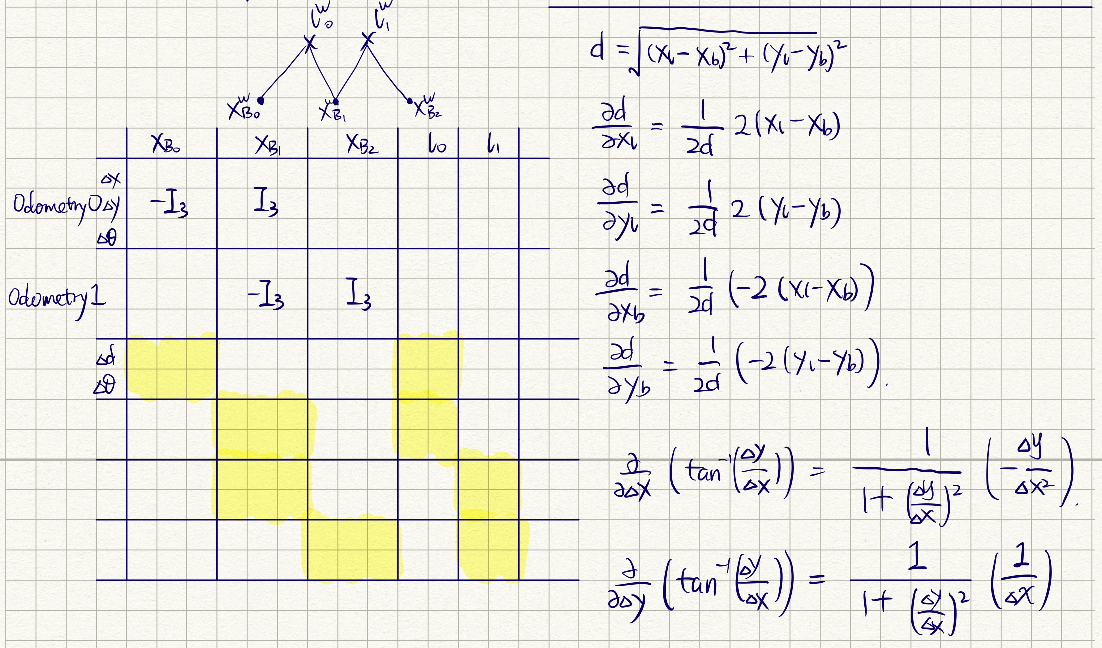
where \(J_k(u_{k:k+L-1})\) accounts for
- control effort \(\sum_{i=1}^L \|u_i\|^2\),
-
robot pose uncertainty (sum of covariance trace),
-
Distance to current goal \(\|X^W_{B_{k + L}} - X^W_{B_{\text{goal}}}\|^2\) + ...
: robot goals.
: landmark ground truths.
: landmark beliefs.
: current robot position (ground truth).
: robot sensing range.
Landmark measurements.
:Robot pose beliefs. \(k\): current time step.
:landmark beliefs.
Additional details:
- Robot dynamics: \( X^W_{B_{i+1}} = X^W_{B_{i}} + u_i \).
- Measurement noises are Gaussian for \(d\) or wrapped Gaussian for \(b\).
: information matrix of current robot pose and landmark beliefs.
Dependencies
Control effort
Pose uncertainty
Distance to goal
Using existing libraries are nice, but...
- iSAM/GTSAM minimizes cost functions of the form \(\|r(x)\|^2\). It seems difficult to massage (41) into a nonlinear least square...
- ROS involves multiple processes communicating with each other though message passing, which makes debugging harder and results non-deterministic.
- As a result, we implemented Active SLAM planner using mostly numpy, with pydrake and pytorch for gradient computation.
- As (41) shares the same Jacobian computation as SLAM Backend, we also implemented SLAM backend as a sanity check.
- Our frontend is simple enough to be implemented with numpy.
We need \(u^*_{k:k+L-1} = \text{argmin} J_k(u_{k:k+L-1})\), where
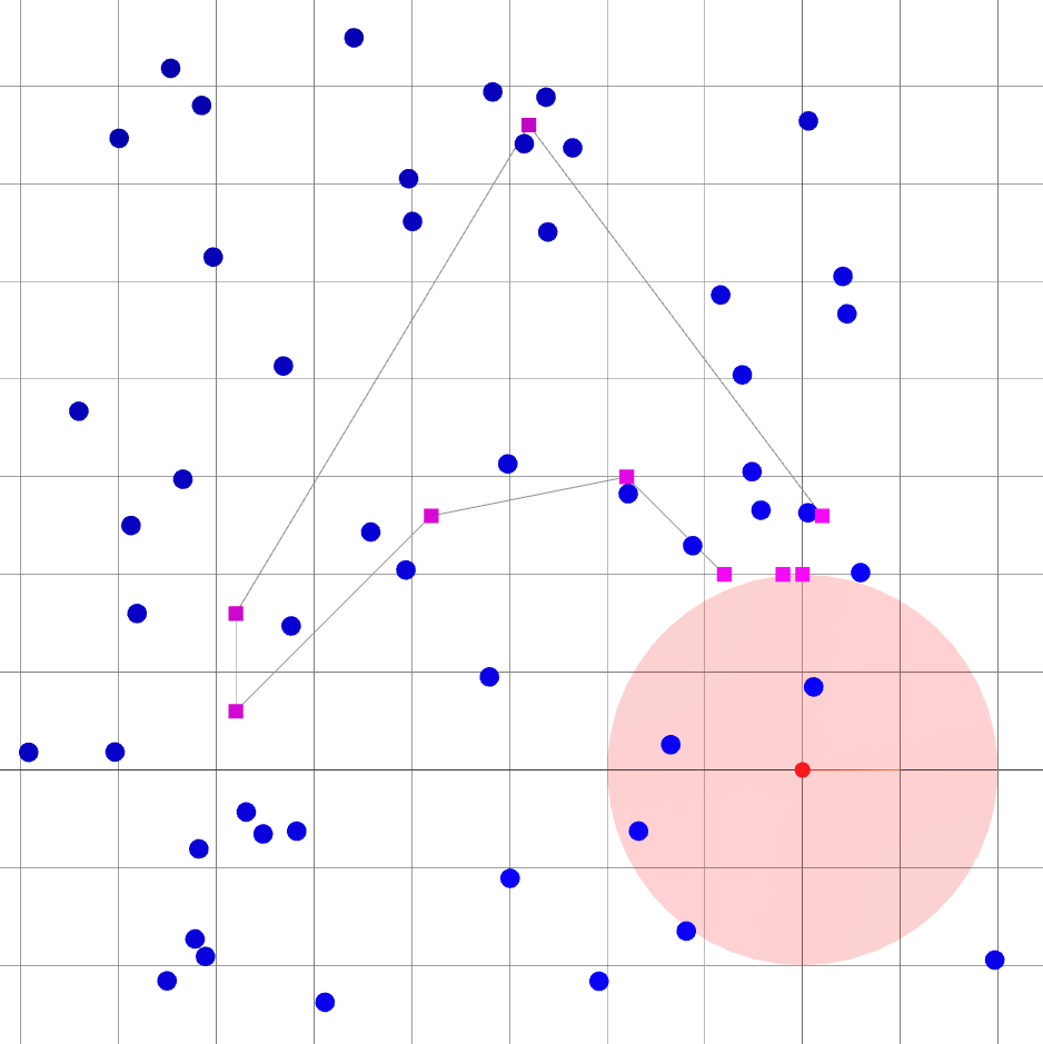
Backend (landmark-based SLAM)
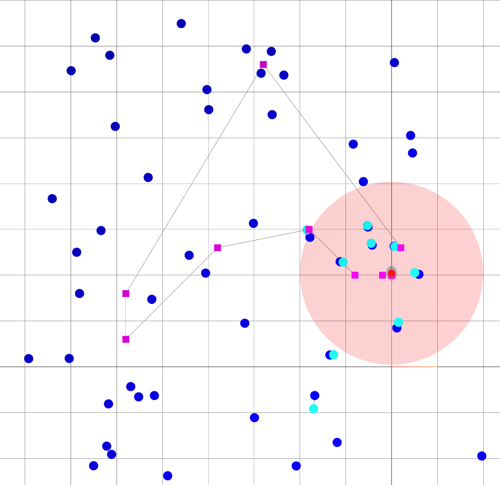
: robot goals.
: landmark ground truths.
: landmark beliefs.
: current robot position (ground truth).
: robot sensing range.
: robot covariance ellipse.
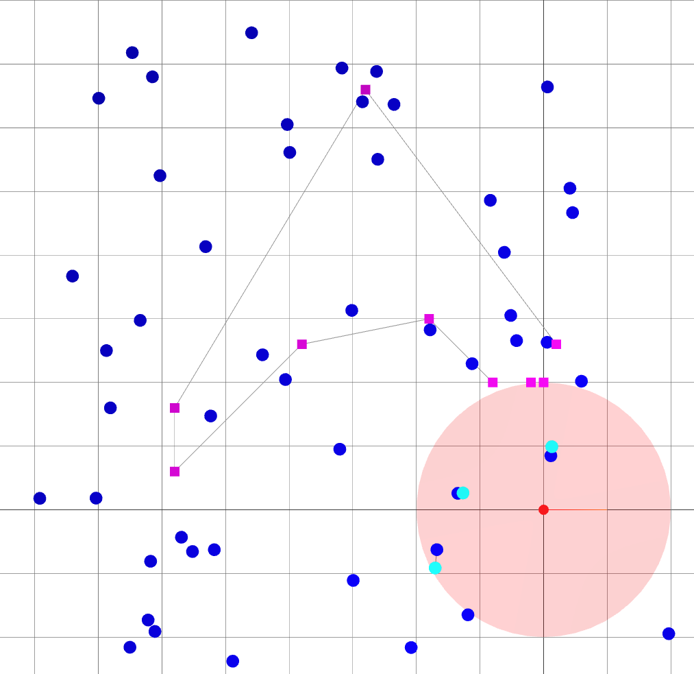
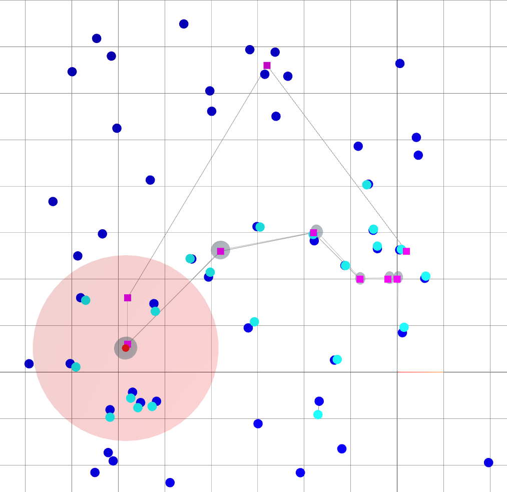
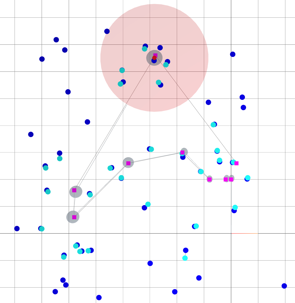
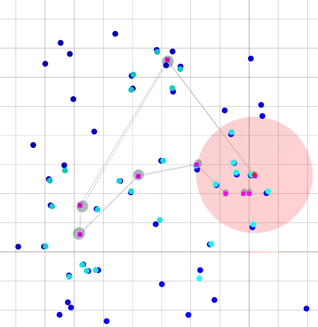
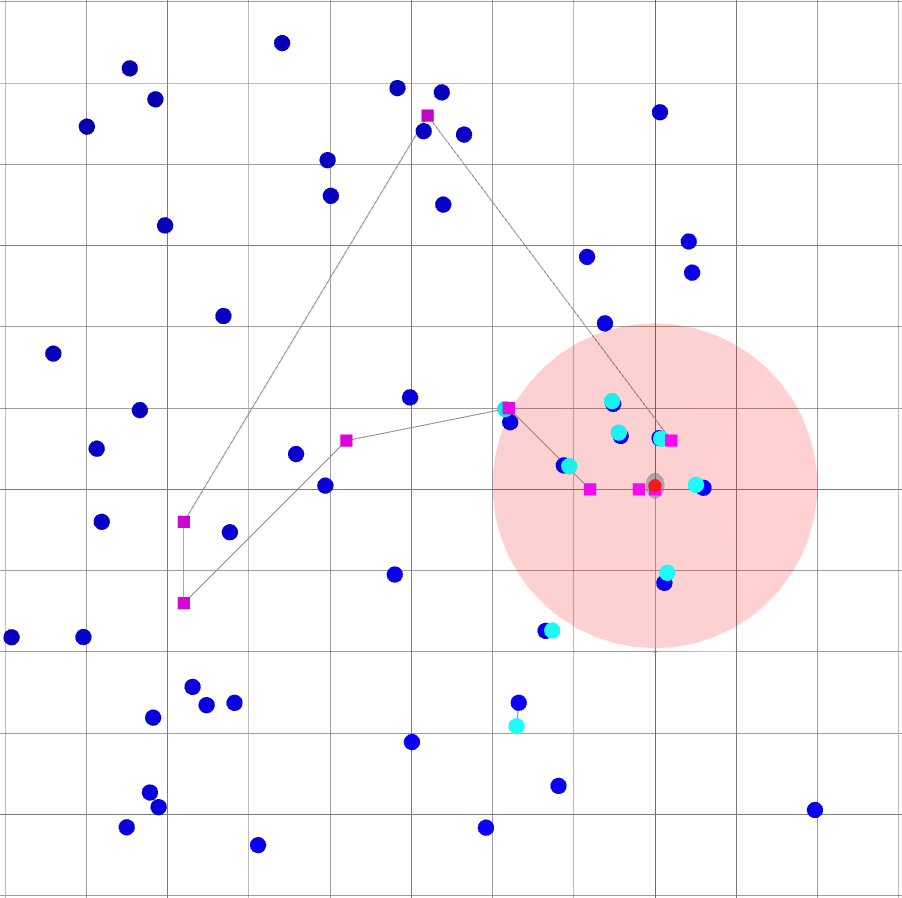
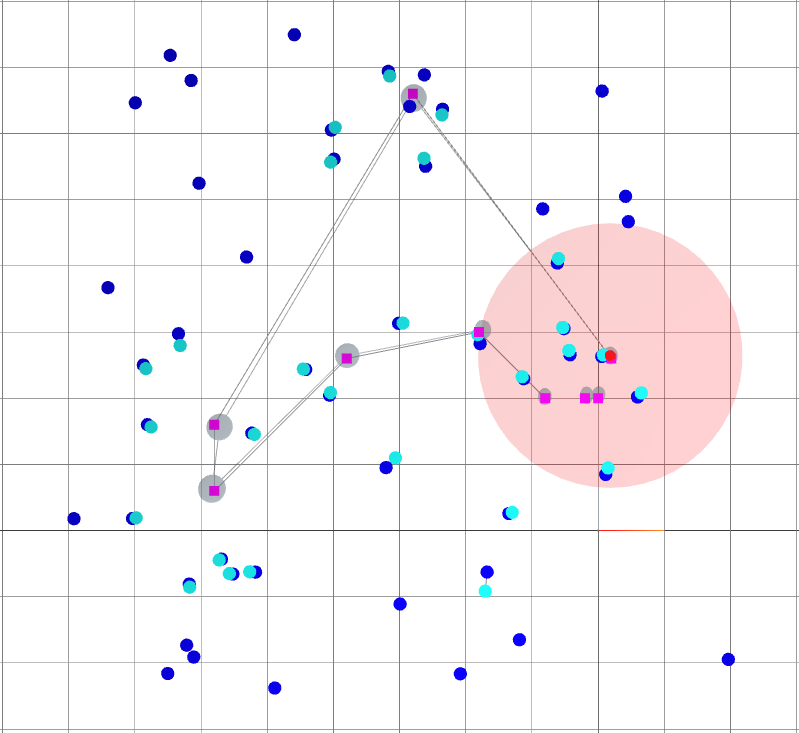
Backend (landmark-based SLAM): Loop closure
: robot goals.
: landmark ground truths.
: landmark beliefs.
: current robot position (ground truth).
: robot sensing range.
: robot covariance ellipse.
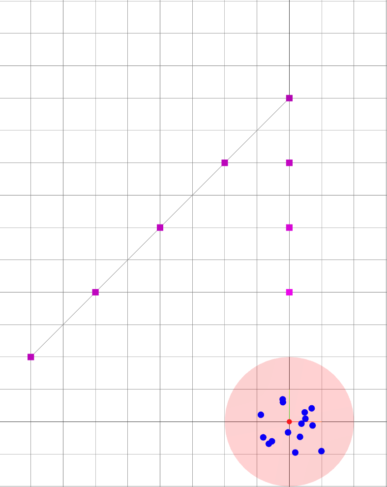
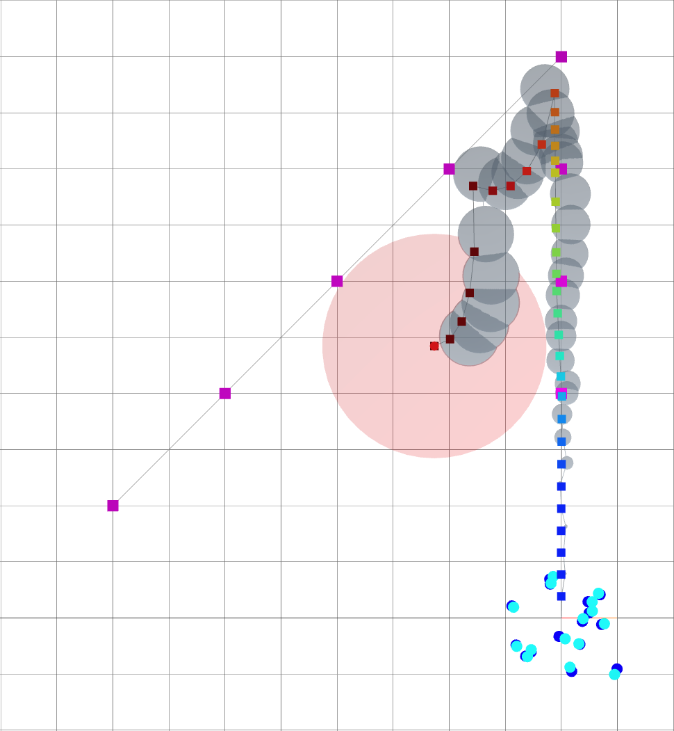
Oasis: map for Active SLAM
- The environment is devoid of landmarks except near the origin.
- Following the given path naively leads to large variance in the robot's belief of its position.
: robot goals.
: landmark ground truths.
: landmark beliefs.
: current robot position (ground truth).
: robot sensing range.
: robot trajectory belief.
: robot trajectory ground truth.

Small \(\alpha\): reaching goal.
Large \(\alpha\): Reducing uncertainty.
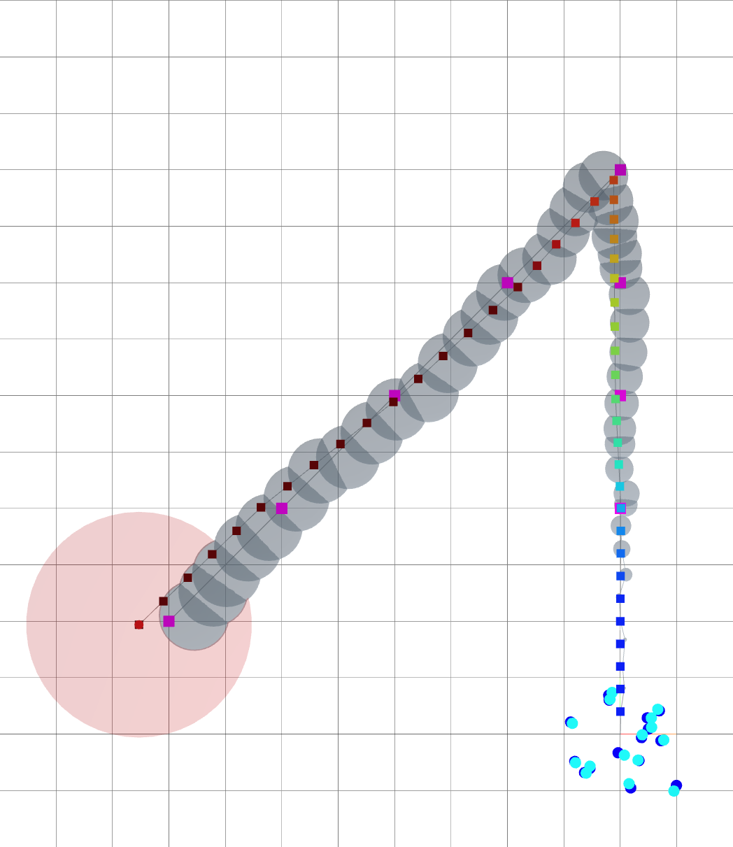
Navigating oasis with Active SLAM
When \(\alpha\) is small, the robot mostly follows the goals.
Small \(\alpha\): reaching goal.
Large \(\alpha\): reducing uncertainty.
time
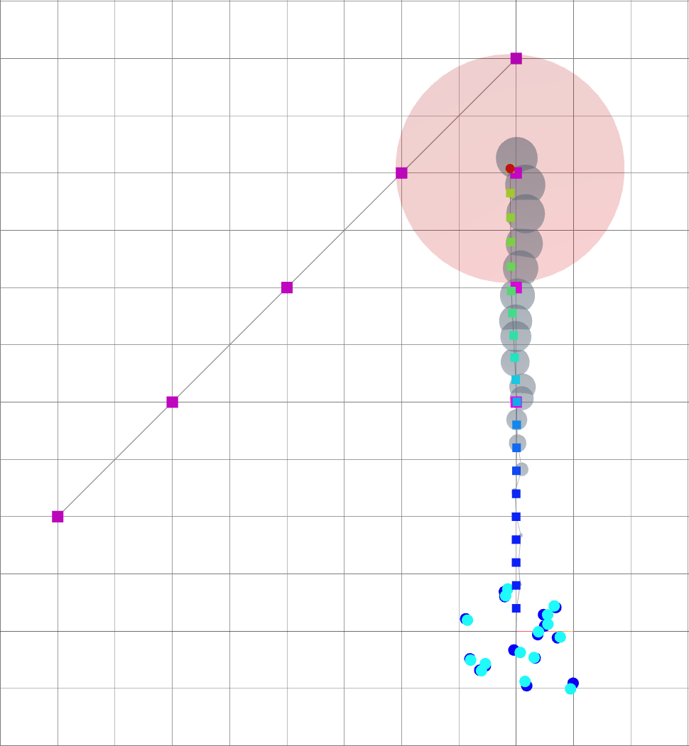
Navigating oasis with Active SLAM
As alpha grows, the robot is driven away from goals and towards landmarks.
Small \(\alpha\): reaching goal.
Large \(\alpha\): reducing uncertainty.
time
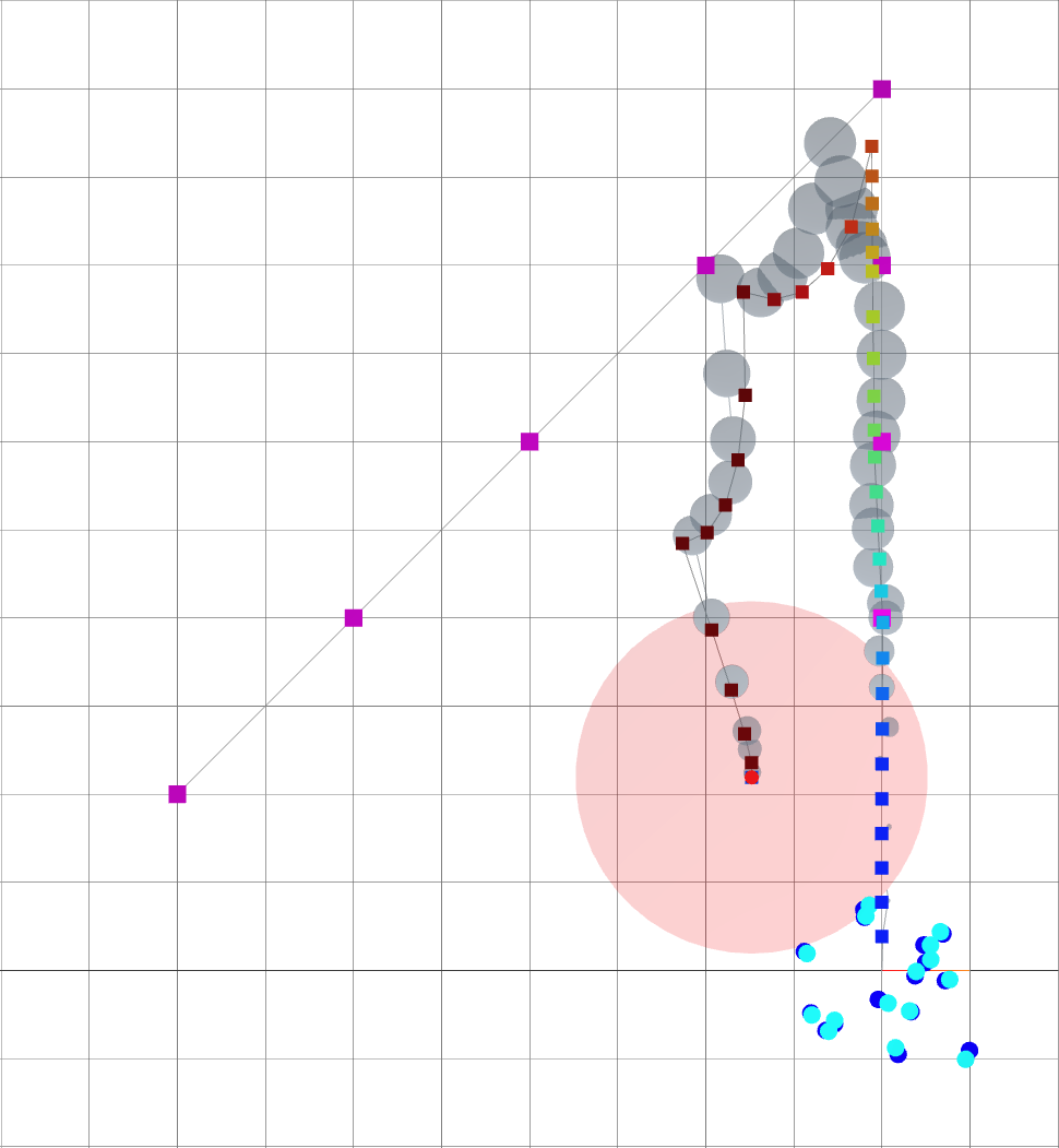
A loop closure is achieved, reducing the variance of the entire trajectory.
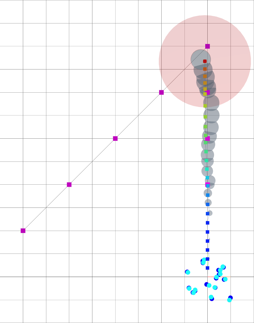
Navigating oasis with Active SLAM
The robot reaches its goal with much smaller variance.
Small \(\alpha\): reaching goal.
Large \(\alpha\): reducing uncertainty.
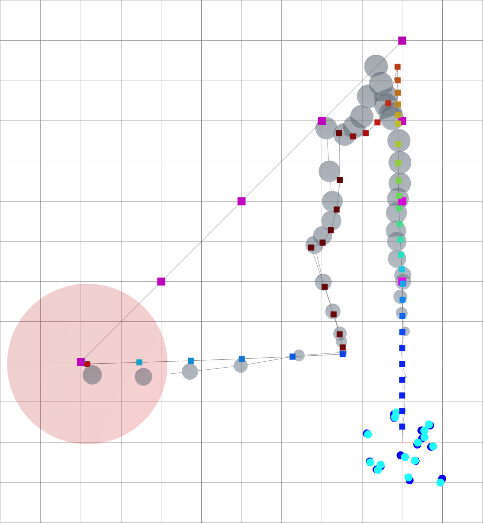
vs.
Without active SLAM.
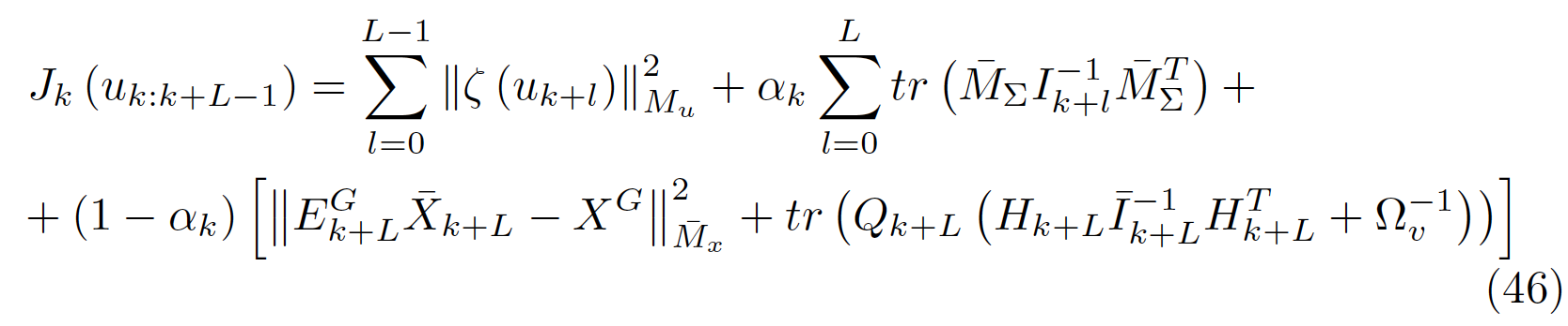
Computing the gradient of \(J_k(u_{k:k+L-1})\)
Control effort
Pose uncertainty
Distance to goal
- Optimizing \(J_k(u_{k:k+L-1})\) is done by gradient descent, therefore we need to compute the gradient quickly.
- We experimented with three ways to compute the gradient of \(J_k(u_{k:k+L-1})\):
- Numerical differentiation.
- Forward-mode automatic differentiation, using Eigen::AutoDiffXd (python bindings provided by pydrake).
- Reverse-mode automatic differentiation, aka backdrop, using pytorch.
Computing \(\nabla_x f(x)\) for \(f(x) : \mathbb{R}^n \rightarrow \mathbb{R}\)
Our objective function \(J_k(u_{k:k+L-1})\) shares the same form as \(f(x)\).
Numerical differentiation
import numpy as np

def calc_derivative_numerical(x, f):
    # derivative of f
    df = np.zeros_like(x)
    n = len(x)
    h = 1e-3

    for i in range(n):
        x_plus = x.copy()
        x_minus = x.copy()
        x_plus[i] += h
        x_minus[i] -= h

        df[i] = (f(x_plus) - f(x_minus)) / 2 / h

    return df
import numpy as np
from pydrake.math import AutoDiffXd as AD

def calc_derivative_forward(x, f):
    n = len(x)

    # initialize array of x with scalar type AD.
    x_ad = np.zeros(n, dtype=object)
    for i in range(n):
        dx_i = np.zeros(n)
        dx_i[i] = 1.
        x_ad[i] = AD(x[i], dx_i)


    # evaluate f with x_ad.
    y_ad = f(x_ad)

    return y_ad.derivatives()
Reverse-mode AutoDiff
import torch

def calc_derivative_reverse(x, f):
    # initialize array of x as tensor.
    x_torch = torch.tensor(x, requires_grad=True)

    # evaluate f with x_torch.
    y_torch = f(x_torch)

    # backprop.
    y_torch.backward()

    return x_torch.grad
Forward-mode AutoDiff
x0 = AD(3, [1, 0])
x1 = AD(4, [0, 1])
y = x0 + x1 # AD(7, [1, 1])
value \(\in \mathbb{R}\)
partial derivatives\(\in \mathbb{R}^n\)
Computes \(f(\cdot)\) \(2n\) times.
Computes \(f(\cdot)\) \(n + 1\) times.
Computes \(f(\cdot)\) \(2\) times.
Gradient of \(J_k(u_{k:k+L-1})\): computation time
\(u_{k:k+L-1} \in \mathbb{R}^{20}\) (\(L=10\)), \(k=1\), 9 landmarks.
- Numerical: 502 ms ± 2.23 ms
- Forward: 35.4 s ± 598 ms (!)
- Backward: 423 ms ± 2.61 ms
Control effort
Pose uncertainty
Distance to goal
- Computation cost grows with the current time \(k\) and the number of observed landmarks.
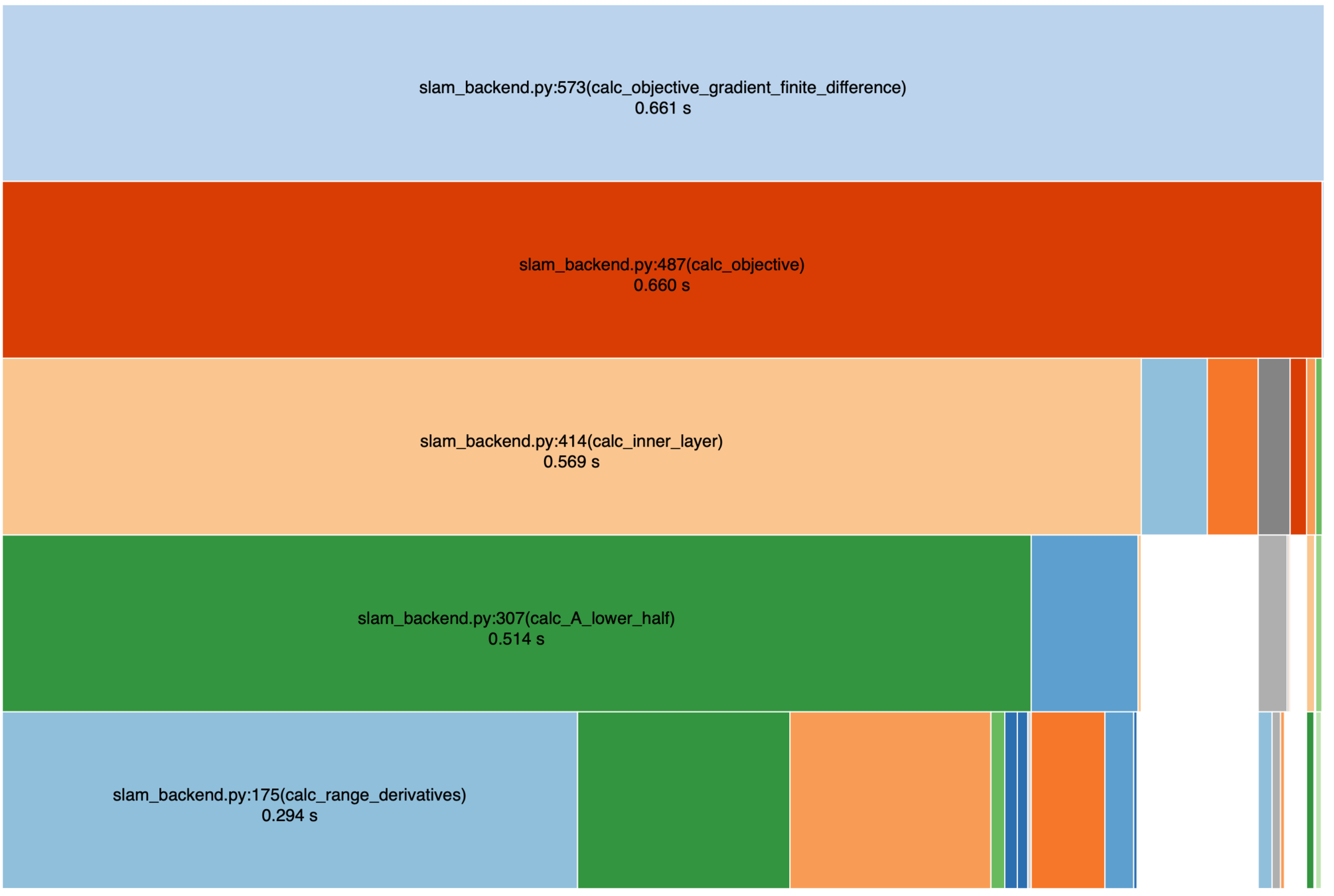
Profiling the computation of \(J_k(u_{k:k+L-1})\)'s gradient: Numerical
Control effort
Pose uncertainty
Distance to goal
Most of the time is spent on computing \(f(\cdot)\), as expected.
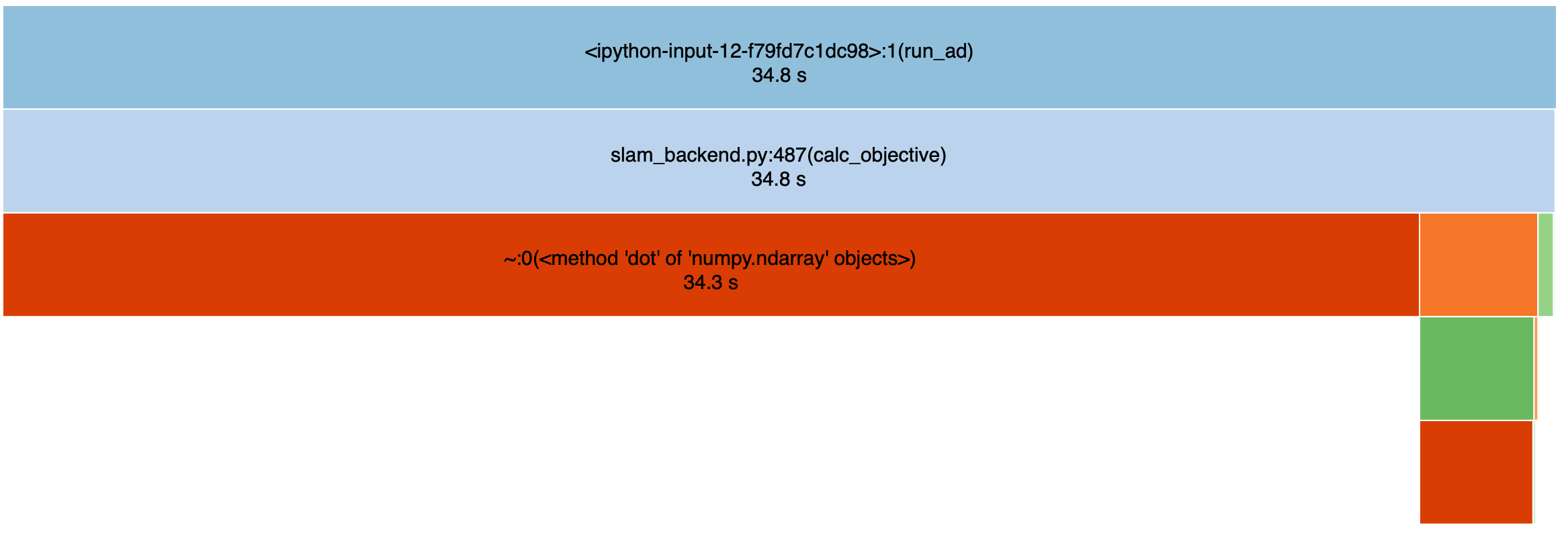
Profiling the computation of \(J_k(u_{k:k+L-1})\)'s gradient: Forward AutoDiff
Control effort
Pose uncertainty
Distance to goal
- Most of the time is spent on matrix multiplication...
- numpy may not have an efficient backend to deal with vectorized operations on AutoDiffXd.
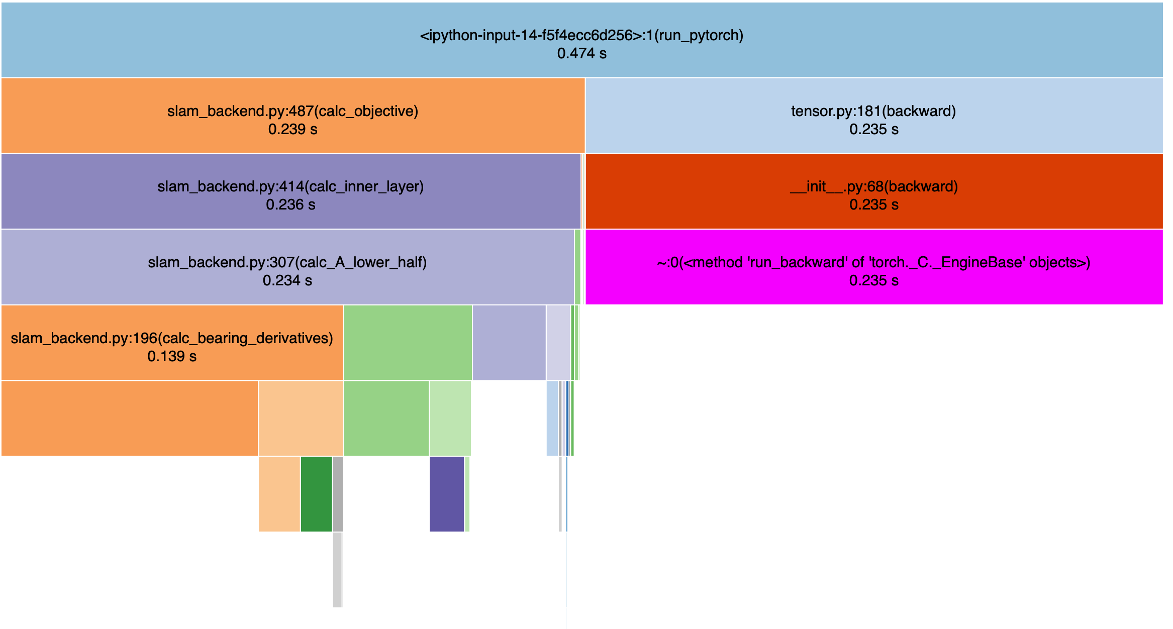
Profiling the computation of \(J_k(u_{k:k+L-1})\)'s gradient: Reverse AutoDiff
Control effort
Pose uncertainty
Distance to goal
Evaluating \(J(u)\) and computing \(\nabla_u J(u)\) takes the same amount of time, as expected.
Computing the gradient of \(J_k(u_{k:k+L-1})\): more complex cases
\(u_{k:k+L-1} \in \mathbb{R}^{20}\) (\(L=10\)), \(k=9\), 28 landmarks.
- Numerical: 1.86 s ± 3.52 ms
- Forward: N.A.
- Backward: 1.42 s ± 3.46 ms
\(u_{k:k+L-1} \in \mathbb{R}^{20}\) (\(L=10\)), \(k=46\), 15 landmarks.
- Numerical: 1.69 s ± 31.1 ms
- Forward: N.A.
- Backward: 754 ms ± 2.35 ms
Making it faster:
- Sparsity
- GPU
Thanks!
- Hold right mouse button: pan.
- Mouse wheel: zoom.
Structure
FrontEnd
-
A 2D robot with two translational DOFs: \(X_B^W = [x, y]\)
-
Noisy measurements of landmarks’ distance \(d\) and bearing \(b\).
BackEnd
- Landmark-based SLAM solved with Levenberg-Marquardt.
Active SLAM with horizon \(L\)
Computes robot control \[u^*_{k:k+L-1} = \text{argmin} J_k(u_{k:k+L-1}),\]
where \(J_k(u_{k:k+L-1})\) accounts for
- control effort,
-
robot pose uncertainty,
-
Distance to current goal.
Landmark measurements.
:Robot pose beliefs.
:landmark beliefs.
Additional details:
- Robot dynamics: \( X^W_{B_{i+1}} = X^W_{B_{i}} + u_i \).
- Measurement noises are Gaussian for \(d\) or wrapped Gaussian for \(b\).
:landmark beliefs.
: information matrix of current beliefs.
:landmark beliefs.
Backend (landmark-based SLAM): Loop closure
: robot goals.
: landmark ground truths.
: landmark beliefs.
: current robot position (ground truth).
: robot sensing range.
: robot covariance ellipse.
Oasis: map for Active SLAM
: robot trajectory belief.
: robot trajectory ground truth.
(a)
(b)
Navigating oasis with Active SLAM
As alpha grows, the robot is driven away from goals and towards landmarks.
Small \(\alpha\): reaching goal.
Large \(\alpha\): reducing uncertainty.
time
A loop closure is achieved, reducing the variance of the entire trajectory.
\(\alpha = 0\)
\(\alpha=1\).