Planning and Control for Contact-rich Manipulation
Pang, Joint work with Terry and Lu
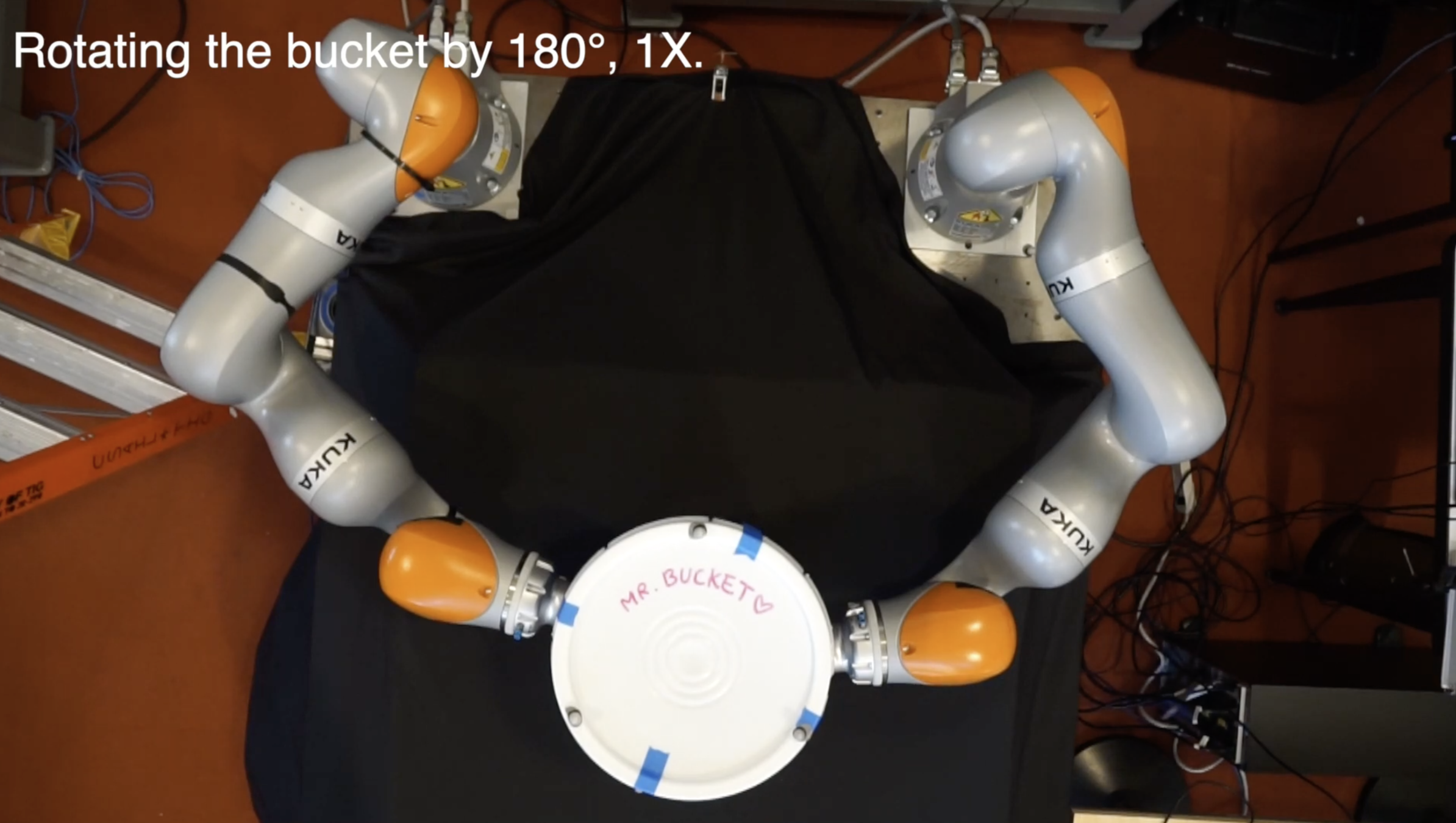
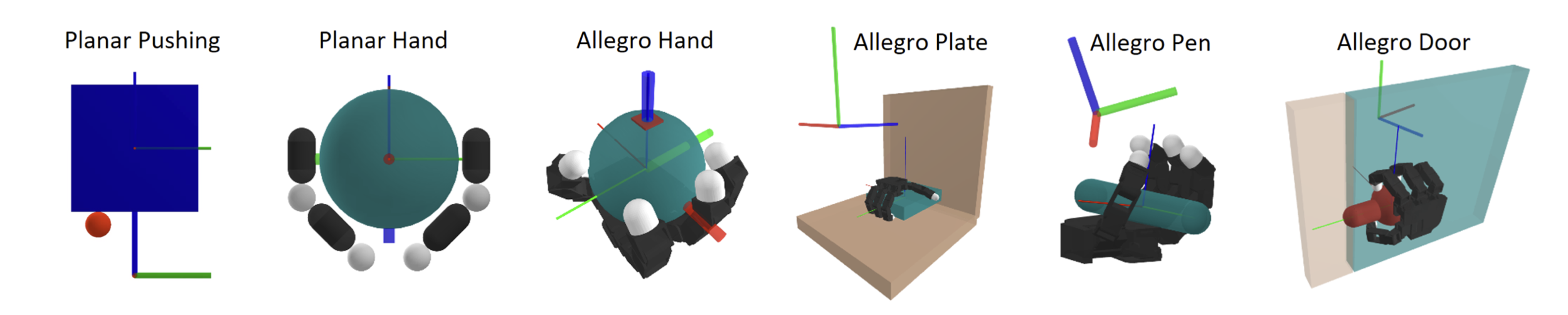
Why contact-rich?
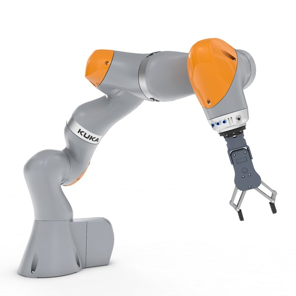
Collision-free Motion Planning
Interact with the world
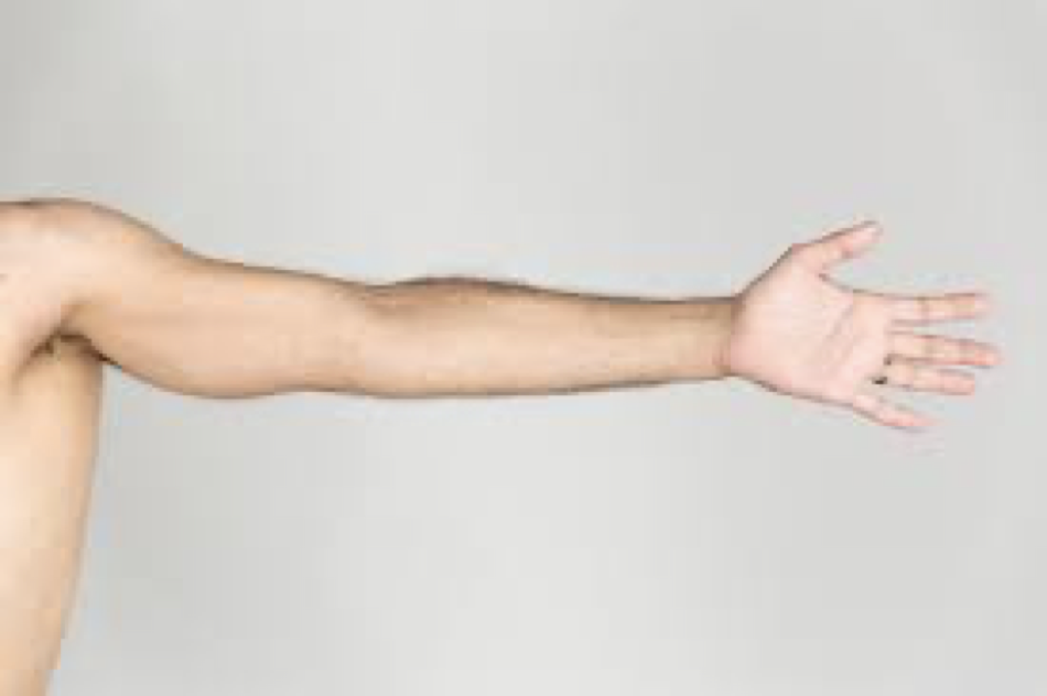
Interact with the world
Collision-free Motion Planning
But this is excessively restrictive!
Why contact-rich?
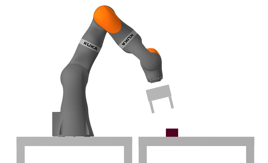
Box

What if we have a larger box...?
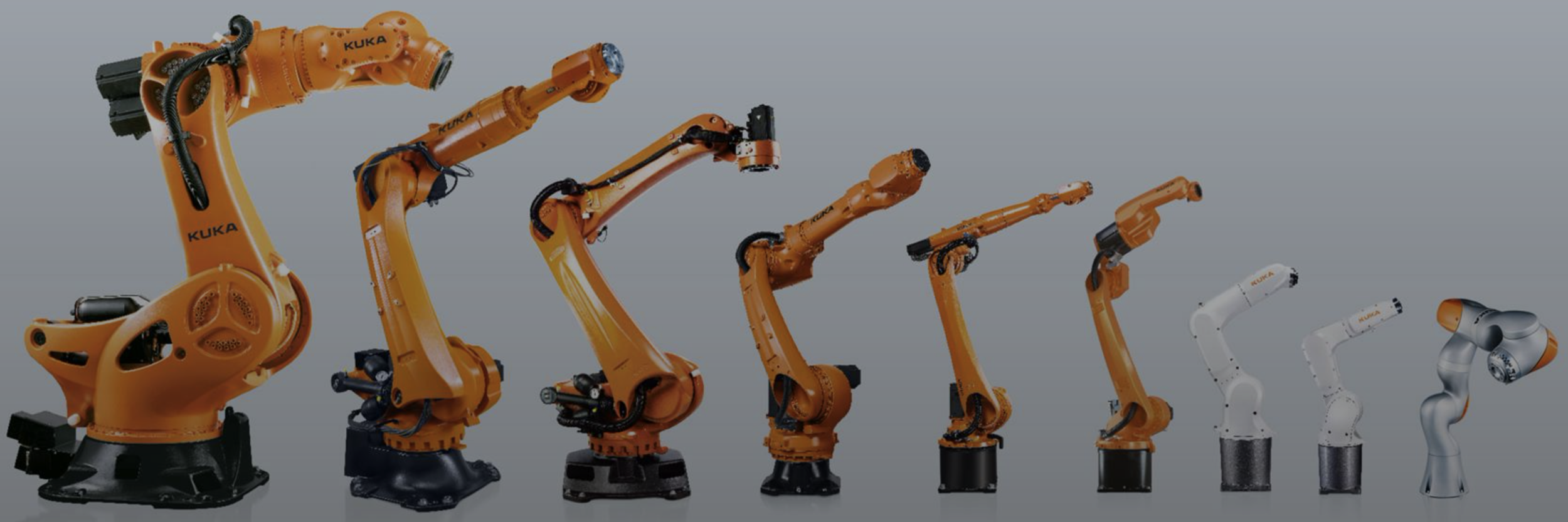
We need to use a bigger arm...
Or make more contacts!
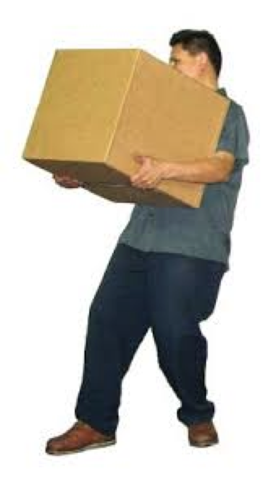
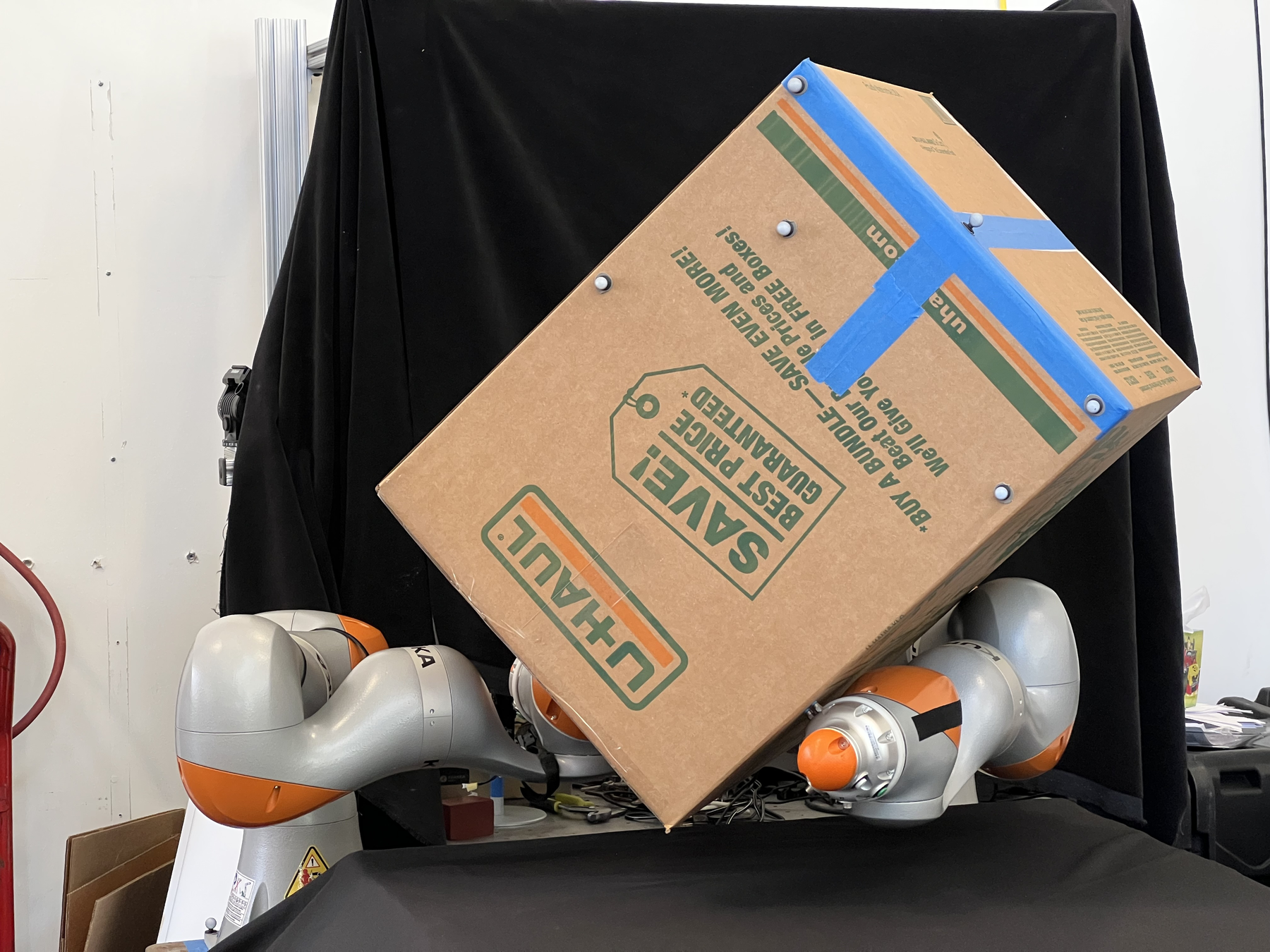
Why contact-rich?
A few more arms
Smaller
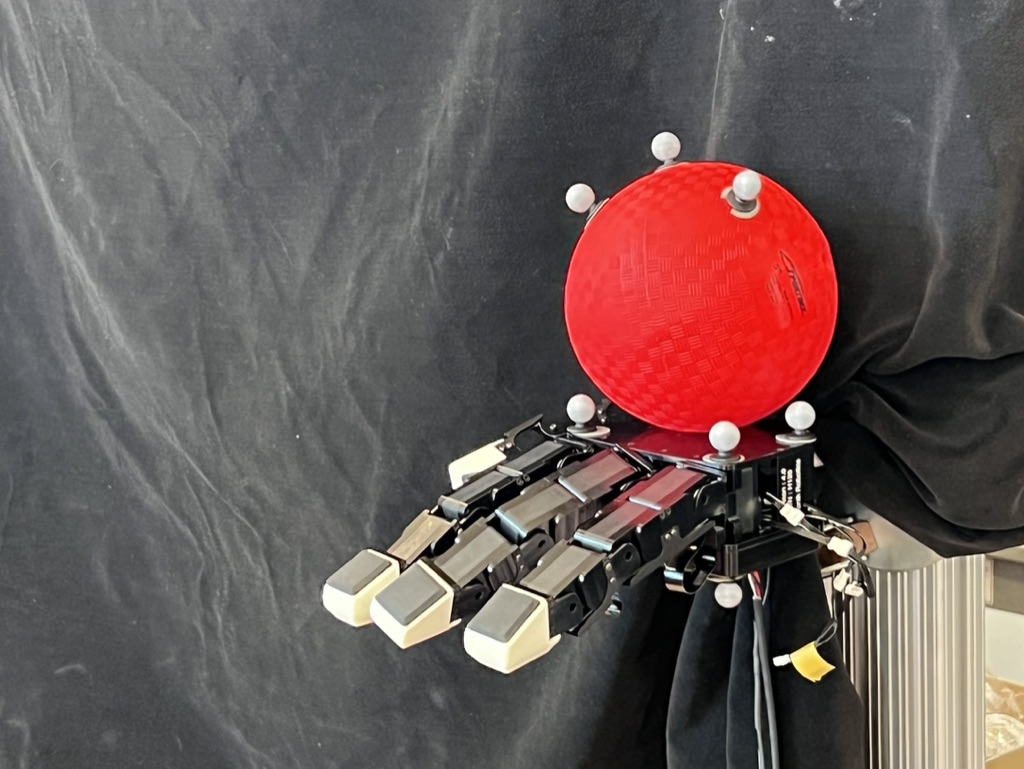
Contact-rich planning and control can enable both bimanual whole-arm manipulation and dexterous manipulation.
Why don't we do RL (reinforcement learning)?
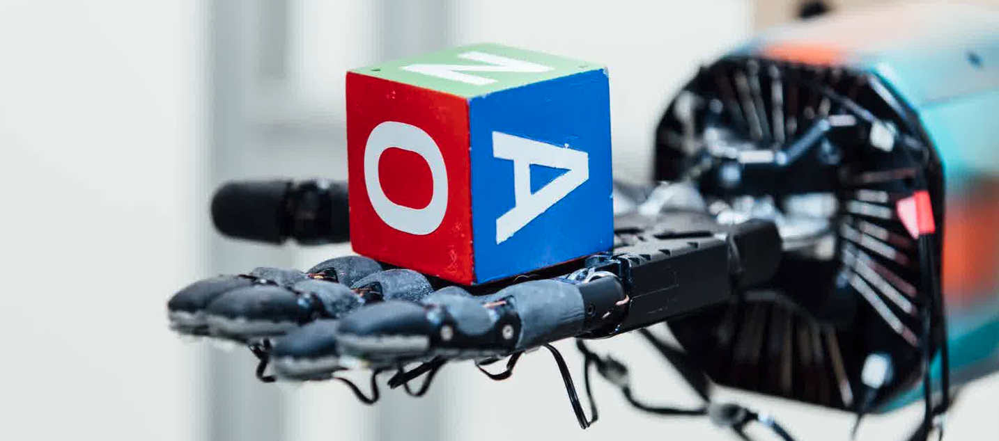
- Impressive demo of in-hand re-orientation, but...
- Excessive offline computation.
- The learned policy
- does not generalize (to e.g. opening a door),
- is hard to interpret.
2018
Model-based Planning through Contact: a Quick Review
2014
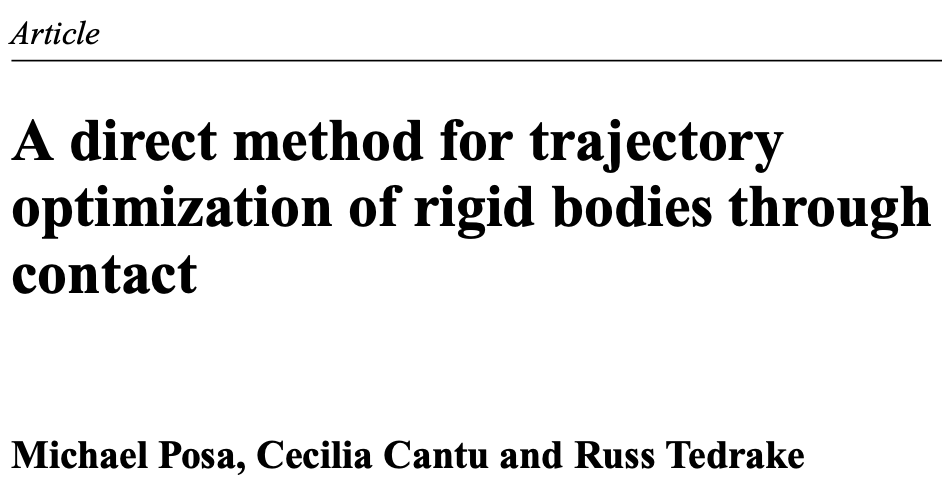
- Nonlinear optimization with
- Lagrangian dynamics constraints.
- Complementarity constraints for frictional contacts.
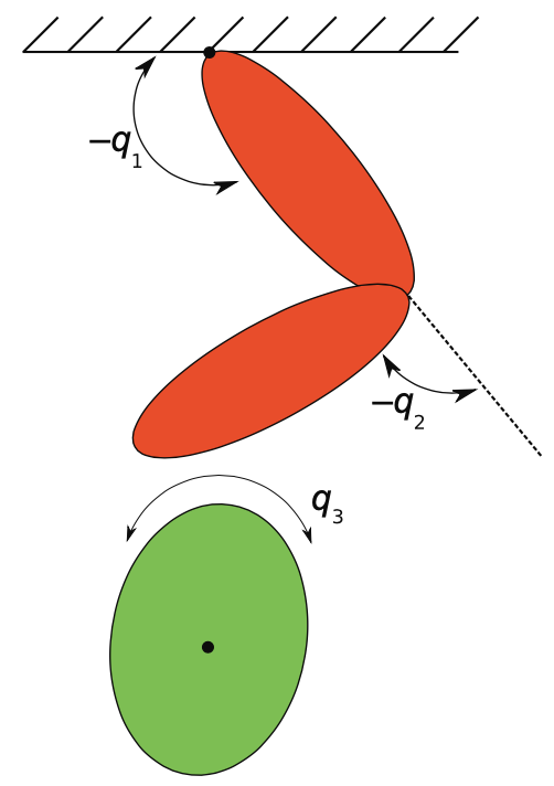

Take aways:
- Traj-opt through contact suffers from local minima, like all other trajectory optimization algorithms.
- PWA + MIP scales poorly with the number of contacts.
2017

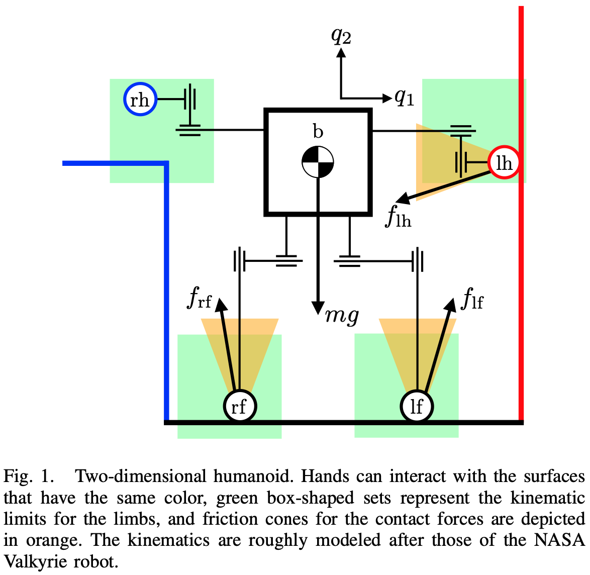
- Model: Piece-wise Affine Systems (PWA)
- Method: Branch and Bound for Mixed-Integer Programming (MIP)
2021

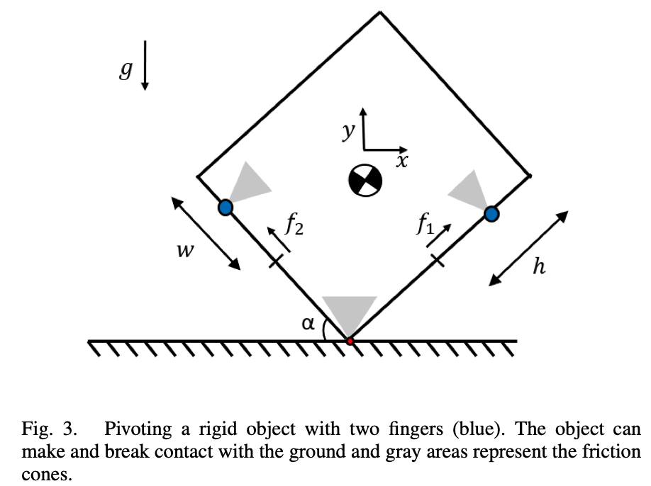
- PWA along a nominal trajectory: fewer pieces.
- Method: specialed ADMM solver for MIP.
But slows down to 16Hz for a more complex system:
2022: Our Method
- RRT and Trajectory optimization for dexterous hands (>16DOF).
- RRT takes less than a minute.
- Trajectory optimization is fast, and only needs trivial initialization.
Open-loop execution of contact-rich plans:
Overview: why did our contact-rich planner work?
- a Convex, Quasi-static Differentiable Simulator
- Quasi-static: \(F = ma\) --> \(F = 0\)
- Convex approximation of contact dynamics (Anitescu).
- Differentiable.
- The model can be easily smoothed.
- Randomized Smoothing --> Deterministic Smoothing (Terry Suh).
- Contact dynamics is non-smooth (\(C^0\)).
- We showed sampling, which RL does a lot, makes contact dynamics smoother (\(C^1\)).
- Our differentiable simulator can be smoothed without sampling, thereby accelerating algorithms that use smoothed gradients.
What does quasi-static mean?
Quasi-static \(\Longleftrightarrow \Sigma F = 0\)
But why is it a good idea?
-
Achieves stable integration with much larger time steps. (0.001s --> 0.4s)
- Ignores transient effects such as damping.
- Considers only transitions between equilibriums.
- Smaller state space (\([q, v]\) vs. only \(q\)).
Second-order
mass matrix
Quasi-static
Coriolis Force
Torque (contact + actuation)
Quasi-static dynamical systems: what it was.
\( x_{+} = f(x, u)\)
- \(x \coloneqq q \coloneqq [q^\mathrm{u}, q^\mathrm{a}]\): system configuration.
- \(q^\mathrm{a}\): actuated, imepdance-controlled robots
- \(q^\mathrm{u}\): un-actuated objects.
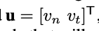
- \( u \): robot velocities.
- Zhou, Jiaji, et al. "A convex polynomial model for planar sliding mechanics: theory, application, and experimental validation." The International Journal of Robotics Research 37.2-3 (2018): 249-265.
- Mason, Matthew T. "Mechanics and planning of manipulator pushing operations." The International Journal of Robotics Research 5.3 (1986): 53-71.
- Hogan, François Robert, and Alberto Rodriguez. "Feedback control of the pusher-slider system: A story of hybrid and underactuated contact dynamics." Algorithmic Foundations of Robotics XII. Springer, Cham, 2020. 800-815.
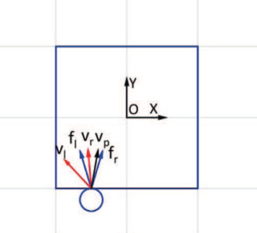
\(\mathrm{v}_p\): applied velocities by the manipulator end effector at the contact point. [1]
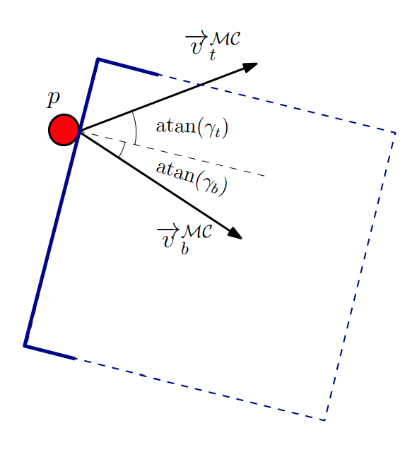
[3]
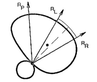
\(R_P\): "the ray of pushing". [2]
This is a good model for planar pushing:
- Contact force cannot be uniquely determined from \(u\) when there is contact.
- As a result, \(q_+\) cannot be determined from \(u\).
- Defining \(u\) as velocity leads to ill-posed dynamical systems (invalid Bond Graphs).
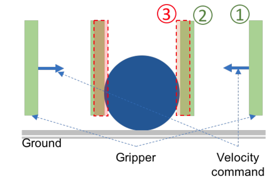
But what about grasping?
Quasi-static dynamical systems: how to fix it.
A Impedance-controlled 1D robot and an object.
- Pang, Tao, and Russ Tedrake. "A convex quasistatic time-stepping scheme for rigid multibody systems with contact and friction." 2021 IEEE International Conference on Robotics and Automation (ICRA). IEEE, 2021.
- Pang, Tao, and Russ Tedrake. "A robust time-stepping scheme for quasistatic rigid multibody systems." 2018 IEEE/RSJ International Conference on Intelligent Robots and Systems (IROS). IEEE, 2018.
\( x_{+} = f(x, u)\)
- \(x \coloneqq q \coloneqq [q^\mathrm{u}, q^\mathrm{a}]\): system configuration.
- \(q^\mathrm{a}\): actuated, imepdance-controlled robots
- \(q^\mathrm{u}\): un-actuated objects.
- \( u \):
robot velocities.position command to the impedance-controlled robots.
Contact force and \(q_+\) can now be uniquely* determined from \(u\), even for grasping.
Force-acceleration vs. Impulse-Momentum
Force-acceleration
- Stewart, David E. "Rigid-body dynamics with friction and impact." SIAM review 42.1 (2000): 3-39.
Impulse-momentum
is the optimality condition of
But impacts can lead to infinite forces (e.g. Painleve's Paradox) [1].
Time step
Quasi-static Dynamics with Contacts
KKT
KKT
: signed distance function.
Robot
Robot
Quasi-dynamic: Quasi-static with Regularization
Quasi-static
- The quadratic cost is semi-definite.
- The object \(m^\mathrm{u}\) can be anywhere on the right of the robot, similar to having a null space.
Robot
Regularized least squares
Regularized Quasi-static
- The quadratic cost is now definite.
- "Among all possible object motions, give me the one that moves the least."
- Picking \(\epsilon = m^\mathrm{u} / h\) gives Mason's definition of quasi-dynamic dynamics.
What about friction?
- For a frictionless multi-body system with \(n_\mathrm{c}\) contacts, the dynamics can be solved as a Quadratic Program (QP):
- \(\mathcal{K}^\star_i\) is the dual of the \(i\)-th friction cone.
- Still convex! Convexity is achieved at the expense of "hydroplaning" between relatively-sliding objects.
- But hydroplaning disappears as \(h \rightarrow 0\).
- Anitescu [1] has a nice convex approximation of Coulomb friction constraints, allowing us to write down the dynamics as a Second-Order Cone Program (SOCP):
Tangential displacements
Dynamics of the 1D system with 1 contact
- Anitescu, Mihai. "Optimization-based simulation of nonsmooth rigid multibody dynamics." Mathematical Programming 105.1 (2006): 113-143.
Differentiability
Convex, Quasi-Dynamic, Differentiable Dynamics (an SOCP)
- The KKT optimality condition of the dynamics SOCP defines equality constraints (including active contact constraints), from which the derivatives of \(\delta q^\star\) w.r.t. \((\mathbf{Q}, b, \phi_i, \mathbf{J}_{\mathrm{n}_i}, \mathbf{J}_{\mathrm{t}_i})\) can be computed using the Implicit Function Theorem (IFT).
- \(\mathbf{A}, \mathbf{B}\) can then be computed using the gradients from IFT and the chain rule.
- Standard practice for many differentiable simulators, even though many of them do not find the active constraints by solving convex programs.
Smoothing
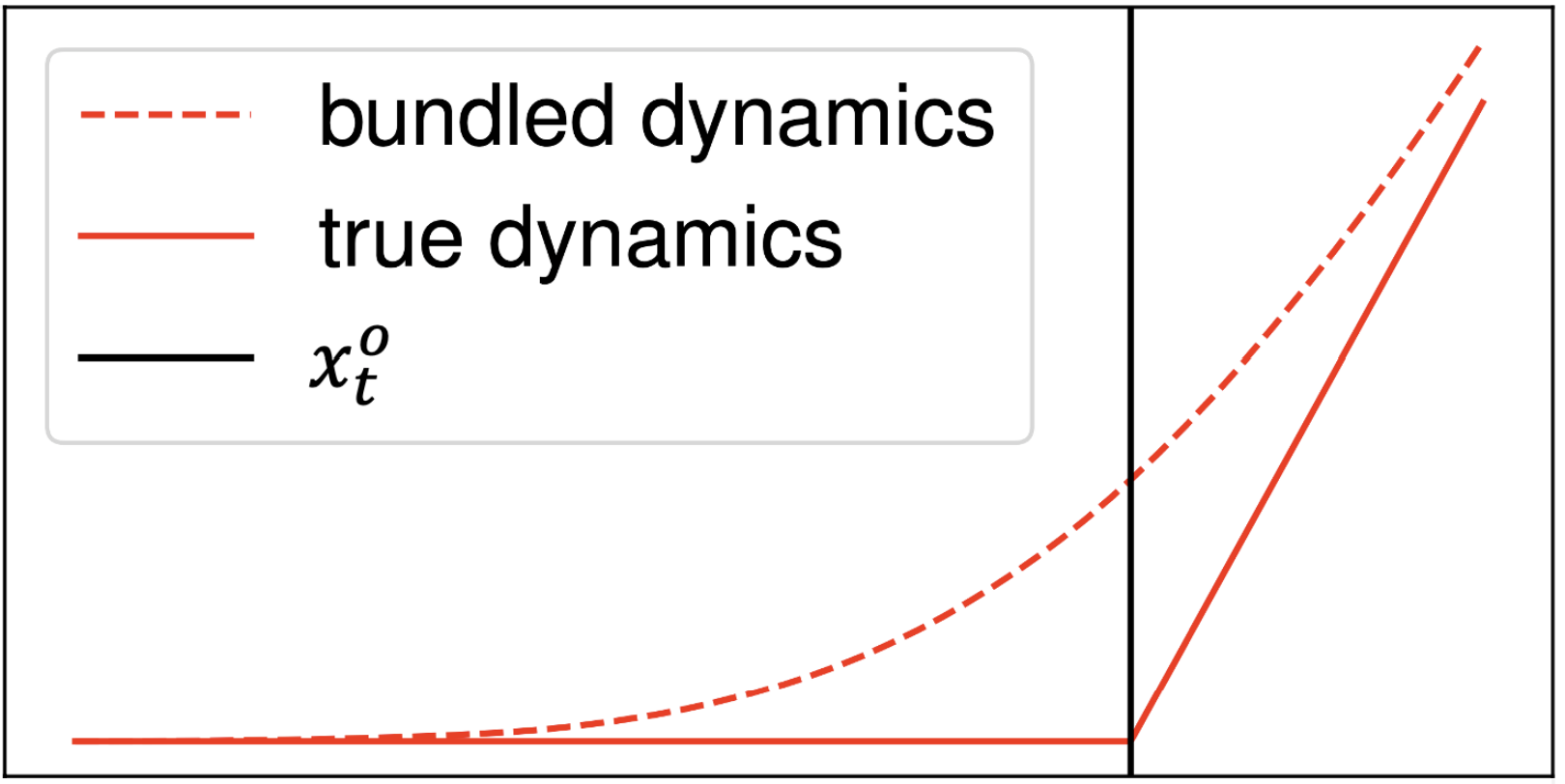
- The contact dynamics \(f(q, u) \in C^0\) has discontinuous gradients, which are bad for planning methods that use gradients.
- Smoothing with "force at a distance" is a common method to alleviate this problem.
smoothed dynamics
original dynamics
\(q^\mathrm{u}\)
Smoothed Dynamics
Optimality Condition
Robot
KKT
Original Dynamics
Smoothing, the general case.
Put constraints in a generalized log for \(\mathcal{\kappa}_i^\star\)
- An unconstrained convex program.
- Can be solved with Newton's method.
- Also differentiable.
Convex, Quasi-Dynamic, Differentiable Dynamics (an SOCP)
Notation:
Original dynamics
Smoothed dynamics
Gradients of the smoothed dynamics enable trajectory optimization for dexterous hands
Task: Turning the ball by 30 degrees.
What about 180 degrees?
RRT is good at escaping local minima, but...
- Kino-dynamic RRT needs a good distance metric! Think about the bycicle.
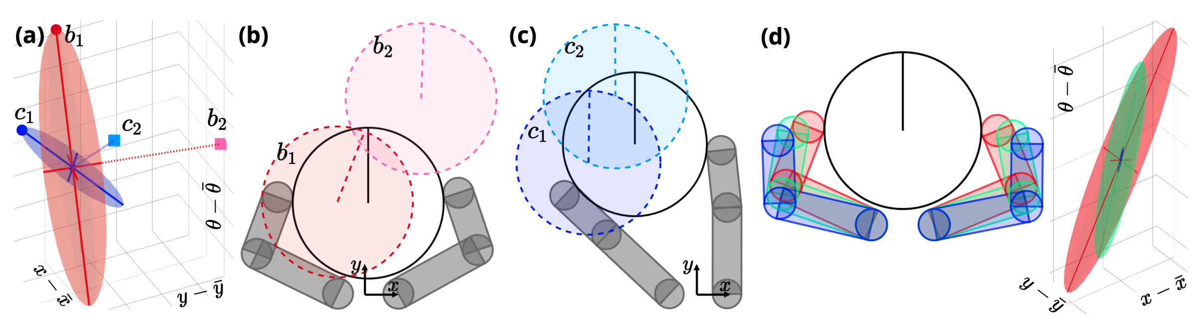
- A good metric from a queried state \(q\) to a nominal state \(\bar{q}\) can be derived based on the smoothed linearization at \(\bar{q}\):
Regularization. \(\gamma\) is small.
\(\varepsilon \) sub-level set
No regularization
Smoothed Contact Dynamics
- \(d^\mathrm{u}_{\rho, \gamma}(q; \bar{q})\) is large (dominated by regularization) when
un-actauted(objects)
Smoothed.
Regularized.
RRT through contact
Motivated by the need of a non-degenerate distance metric, two modifications to the vanilla RRT are made:
- Connect: the nearest node on the tree to a sample \(q\) is computed using \( d^\mathrm{u}_{\rho, \gamma}(q; \bar{q}) \)
- Contact sampling: with a non-zero probability, robot configuration is reset to one that has a good distance metric, which typically corresponds to grasps.
These modifications, together with smoothing, are essential for efficient state space exploration:
Distance Metric
RRT tree fro a simple system with contacts
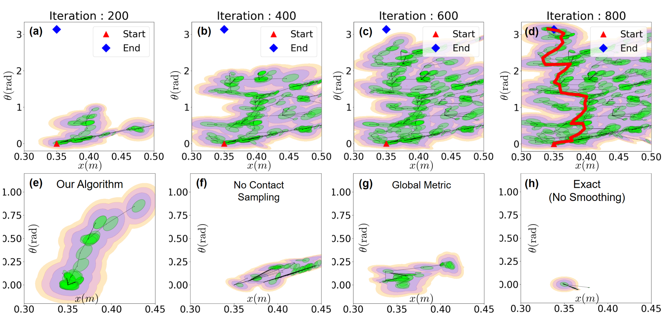
Ablation study: what trees look like after growing a fixed number of nodes.
The modified RRT works well for several systems!


Planning wall-clock time (seconds)
Smoothing by sampling
Smoothing directly
Stabilizing contact-rich plans
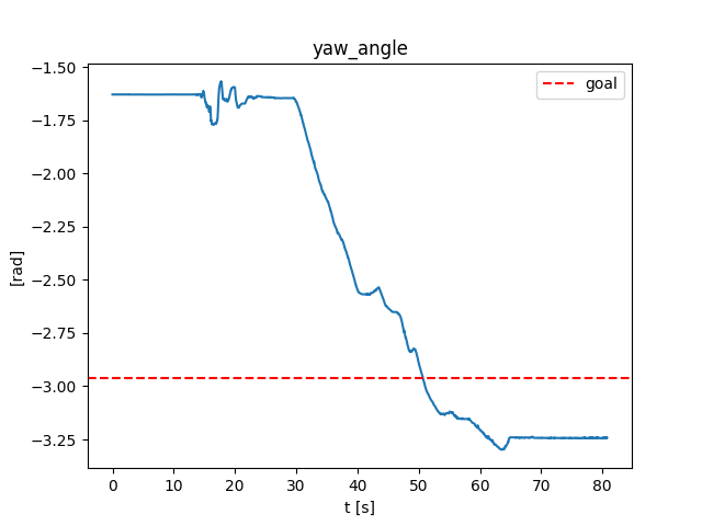
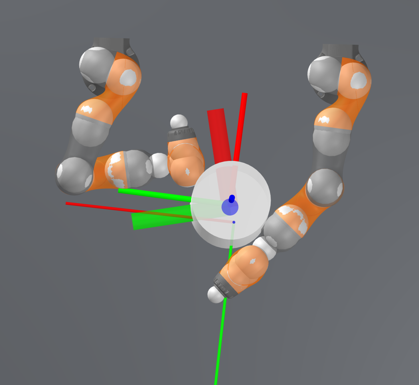
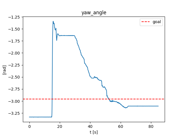
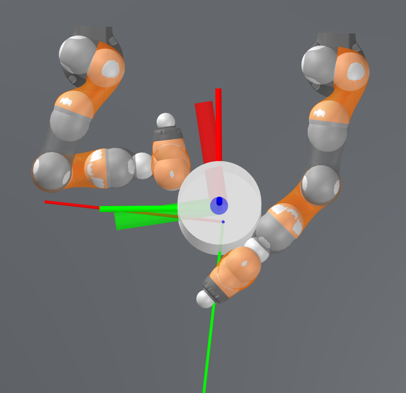
Open-loop
Closed-loop
Goal
Start
Final
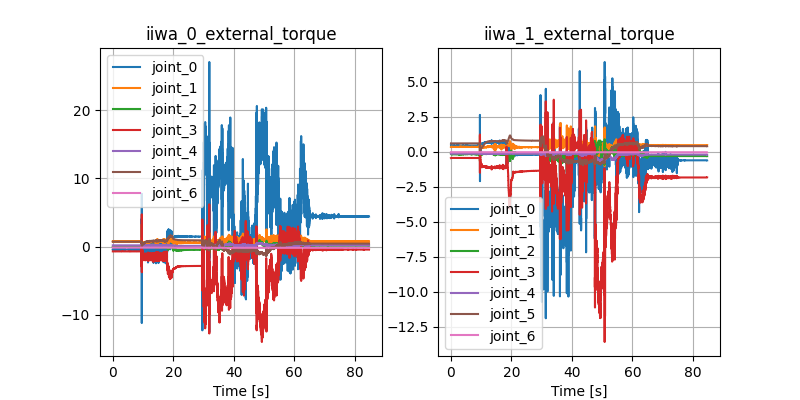
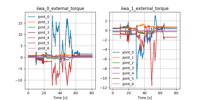
Stabilizing contact-rich plans
Open-loop hardware
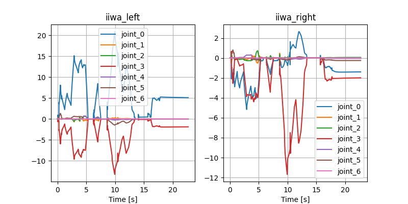
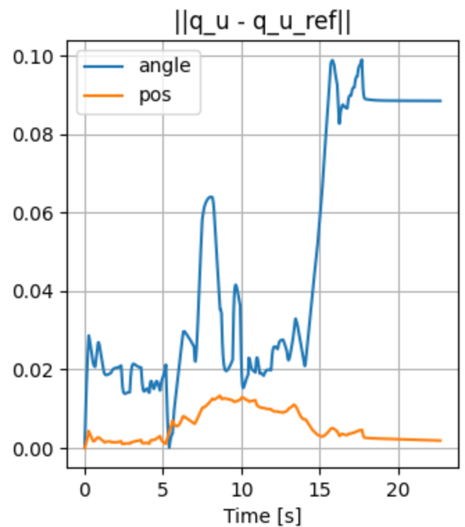
Open-loop Drake
Controller
- Simple (and probably wrong) controller:
Smooth linearization
- Consider modes?
- Tracking joint torque?