A double-covered
probabilistic ray-based
neural shape representation

Peder Bergebakken Sundt
Theoharis Theoharis
3DOR 2026

A double-covered
probabilistic ray-based
neural shape representation
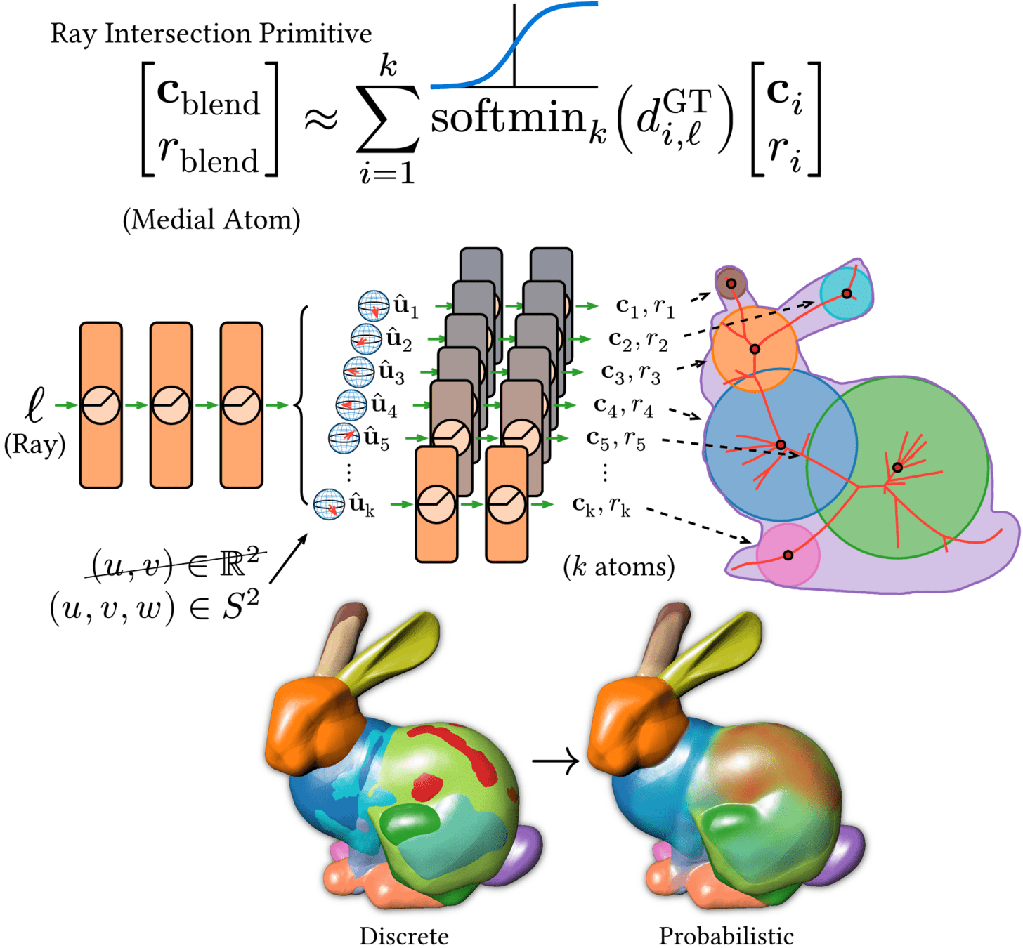
3DOR 2026
A double-covered
probabilistic ray-based
neural shape representation
3DOR 2026
A double-covered
probabilistic ray-based
neural shape representation
3DOR 2026
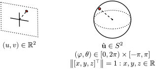
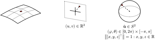
A double-covered
probabilistic ray-based
neural shape representation
3DOR 2026
A double-covered
probabilistic ray-based
neural shape representation
3DOR 2026
- Motivation & Preliminaries
- Contributions
- Results
Why?
Where?
What?
Neural Ray Fields
Motivating
Differentiable rendering requires good gradient flow
Why?
Where?
Primitives
Neural Ray Fields
What?
- Analytical gradients
- Approximate gradients
- Approximate rendering
Differentiable rendering requires good gradient flow
Neural Fields
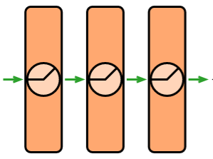
Approximate representations?
Motivating
Why?
Where?
Primitives
Neural Ray Fields
What?
Motivation
- Analytical gradients
- Approximate gradients
- Approximate rendering
- "Coordinate-based" neural network
- Map spatial coordinate to some reconstruction signal.
- Multiple evaluations to sample the reconstruction domain
- DeepSDF, NeRF, NGP
Neural Fields
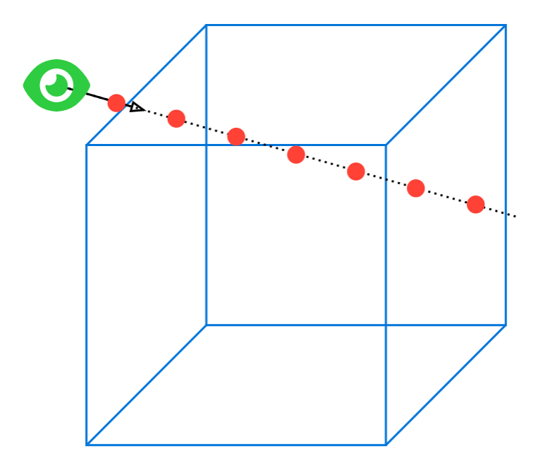
why pick one over the other?
Approximate representations?
Differentiable rendering requires good gradient flow
Why?
Where?
Primitives
Neural Ray Fields
What?
Motivation
- Analytical gradients
- Approximate gradients
- Approximate rendering
why pick one over the other?
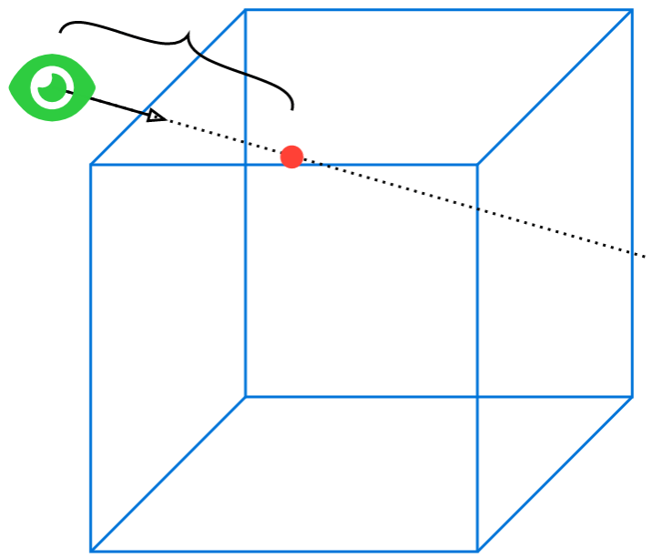
Neural Ray Fields
Neural Fields
- Single evaluation per ray
Differentiable rendering requires good gradient flow
Why?
Where?
Primitives
Neural Ray Fields
What?
Motivation
Neural Fields
Why pick one over the other?
The current SOTA
feature great render times.
Why?
Minimize primitive processing
Minimize network evaluations
Image Diffusion
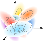
3D Gaussian Splatting
Voxel Grids
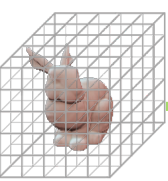
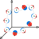
Fast Dipole Sums
Implicit Surface / Radiance Fields
Ray Intersection / Light Fields
Ratio tracking
Edge-sampling
Rasterization
Ray Marching
Ray Casting
Neural Fields
Primitives
Speedup
Where?
Neural Ray Fields

What?
(closed-form solution)
(iterative solution)
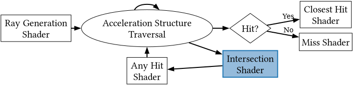
Neural Ray fields are compact and feature non-diverging memory access,
making them attractive as intersection
shaders in hybrid path-tracing
Figure:
The Vulkan Ray-Tracing Pipeline
Neural Ray Fields
Where?
Why?
Related Works
A simplified timeline
Related Works
PRIF
MARF
PMARF
PDDF
LFN
Light Fields
Intersection Fields
NFD
AutoInt
5D
4D
5D
4D
𝒩-BVH
LSNIF
Hybrid
SRDF
Hybrid
- [AutoInt] Lindell DB, Martel JNP, Wetzstein G. AutoInt: Automatic Integration for Fast Neural Volume Rendering. Proceedings of the conference on computer vision and pattern recognition (CVPR), Nashville, TN, USA: IEEE; 2021, p. 14551–60.
- [LFN] Sitzmann V, Rezchikov S, Freeman B, Tenenbaum J, Durand F. Light field networks: Neural scene representations with single-evaluation rendering. Advances in Neural Information Processing Systems 2021;34:19313–25.
- [PRIF] Feng BY, Zhang Y, Tang D, Du R, Varshney A. PRIF: Primary Ray-Based Implicit Function. In: Avidan S, Brostow G, Cissé M, Farinella GM, Hassner T, editors. Computer Vision – ECCV 2022, vol. 13663, Cham: Springer Nature Switzerland; 2022, p. 138–55.
- [MARF] Sundt PB, Theoharis T. MARF: The Medial Atom Ray Field object representation. Computers & Graphics 2023;115:122–36.
- [PMARF] Sundt PB, Theoharis T. Towards multi-view consistency in neural ray fields using parametric medial surfaces. Computers & Graphics 2024;123:103991.
- [NFD] Rebain D, Yazdani S, Yi KM, Tagliasacchi A. Neural fields as distributions: Signal processing beyond Euclidean space. In 2024 IEEE/CVF Conference on Computer Vision and Pattern Recognition (CVPR) 2024 Jun 16 (pp. 4274-4283). IEEE.
- [PDDF] Aumentado-Armstrong T, Tsogkas S, Dickinson S, Jepson A. Probabilistic Directed Distance Fields for Ray-Based Shape Representations. IEEE Transac-tions on Pattern Analysis and Machine Intelligence 2025;47:10243–61.
- [SRDF] Zins P, Xu Y, Boyer E, Wuhrer S, Tung T. Multi-View Reconstruction Using Signed Ray Distance Functions (SRDF). 2023 IEEE/CVF Conference on Computer Vision and Pattern Recognition (CVPR), Vancouver, BC, Canada: IEEE; 2023, p. 16696–706.
- [𝒩-BVH] Weier P, Rath A, Michel É, Georgiev I, Slusallek P, Boubekeur T. N-BVH: Neural ray queries with bounding volume hierarchies. InACM SIGGRAPH 2024 conference papers 2024 Jul 13 (pp. 1-11).
- [LSNIF] Fujieda S, Kao CC, Harada T. LSNIF: Locally-Subdivided Neural Intersection Function. Proceedings of the ACM on Computer Graphics and Interactive Techniques. 2025 May 22;8(1):1-8.
A simplified timeline
Orthogonal to our work.
Plücker
embeddings
Plücker
embeddings
Hybrid
PRIF
MARF
PMARF
PDDF
LFN
This Work
Light Fields
Intersection Fields
NFD
AutoInt
5D
4D
5D
4D
𝒩-BVH
LSNIF
Hybrid
SRDF
Hybrid
- [AutoInt] Lindell DB, Martel JNP, Wetzstein G. AutoInt: Automatic Integration for Fast Neural Volume Rendering. Proceedings of the conference on computer vision and pattern recognition (CVPR), Nashville, TN, USA: IEEE; 2021, p. 14551–60.
- [LFN] Sitzmann V, Rezchikov S, Freeman B, Tenenbaum J, Durand F. Light field networks: Neural scene representations with single-evaluation rendering. Advances in Neural Information Processing Systems 2021;34:19313–25.
- [PRIF] Feng BY, Zhang Y, Tang D, Du R, Varshney A. PRIF: Primary Ray-Based Implicit Function. In: Avidan S, Brostow G, Cissé M, Farinella GM, Hassner T, editors. Computer Vision – ECCV 2022, vol. 13663, Cham: Springer Nature Switzerland; 2022, p. 138–55.
- [MARF] Sundt PB, Theoharis T. MARF: The Medial Atom Ray Field object representation. Computers & Graphics 2023;115:122–36.
- [PMARF] Sundt PB, Theoharis T. Towards multi-view consistency in neural ray fields using parametric medial surfaces. Computers & Graphics 2024;123:103991.
- [NFD] Rebain D, Yazdani S, Yi KM, Tagliasacchi A. Neural fields as distributions: Signal processing beyond Euclidean space. In 2024 IEEE/CVF Conference on Computer Vision and Pattern Recognition (CVPR) 2024 Jun 16 (pp. 4274-4283). IEEE.
- [PDDF] Aumentado-Armstrong T, Tsogkas S, Dickinson S, Jepson A. Probabilistic Directed Distance Fields for Ray-Based Shape Representations. IEEE Transac-tions on Pattern Analysis and Machine Intelligence 2025;47:10243–61.
- [SRDF] Zins P, Xu Y, Boyer E, Wuhrer S, Tung T. Multi-View Reconstruction Using Signed Ray Distance Functions (SRDF). 2023 IEEE/CVF Conference on Computer Vision and Pattern Recognition (CVPR), Vancouver, BC, Canada: IEEE; 2023, p. 16696–706.
- [𝒩-BVH] Weier P, Rath A, Michel É, Georgiev I, Slusallek P, Boubekeur T. N-BVH: Neural ray queries with bounding volume hierarchies. InACM SIGGRAPH 2024 conference papers 2024 Jul 13 (pp. 1-11).
- [LSNIF] Fujieda S, Kao CC, Harada T. LSNIF: Locally-Subdivided Neural Intersection Function. Proceedings of the ACM on Computer Graphics and Interactive Techniques. 2025 May 22;8(1):1-8.
Related Works
A simplified timeline
We iterate on MARF and PMARF, with some improvements
inspired by NFD and PDDF, and some novel.
View overfitting
The 5 (or 4) degrees-of-freedom in rays
permit view-dependent geometry.
The primary challenge:
You can alleviate view overfitting with
dense multi-view supervision.
...but can one do without?
Early work
⇒ Multi-view consistent priors
and regularization
Overfitting on purpose is a no-go.
(Medial Atom) Ray Fields
A quick refresher
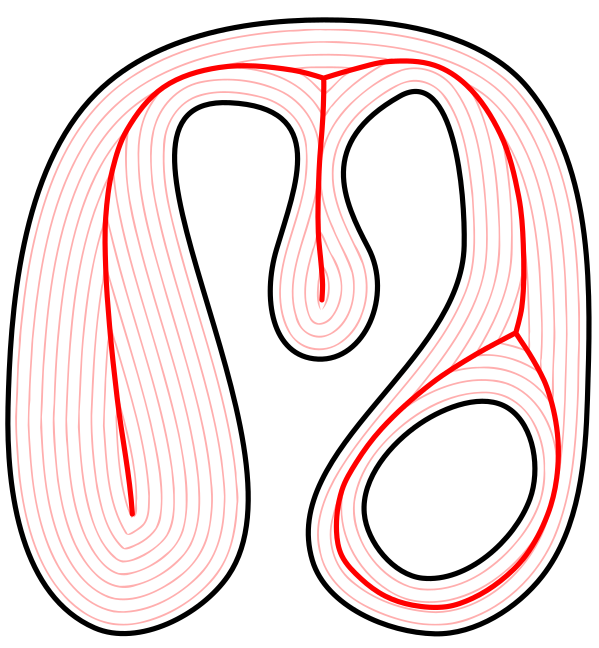
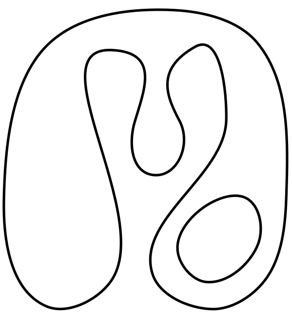
shape
A quick refresher
(Medial Atom) Ray Fields
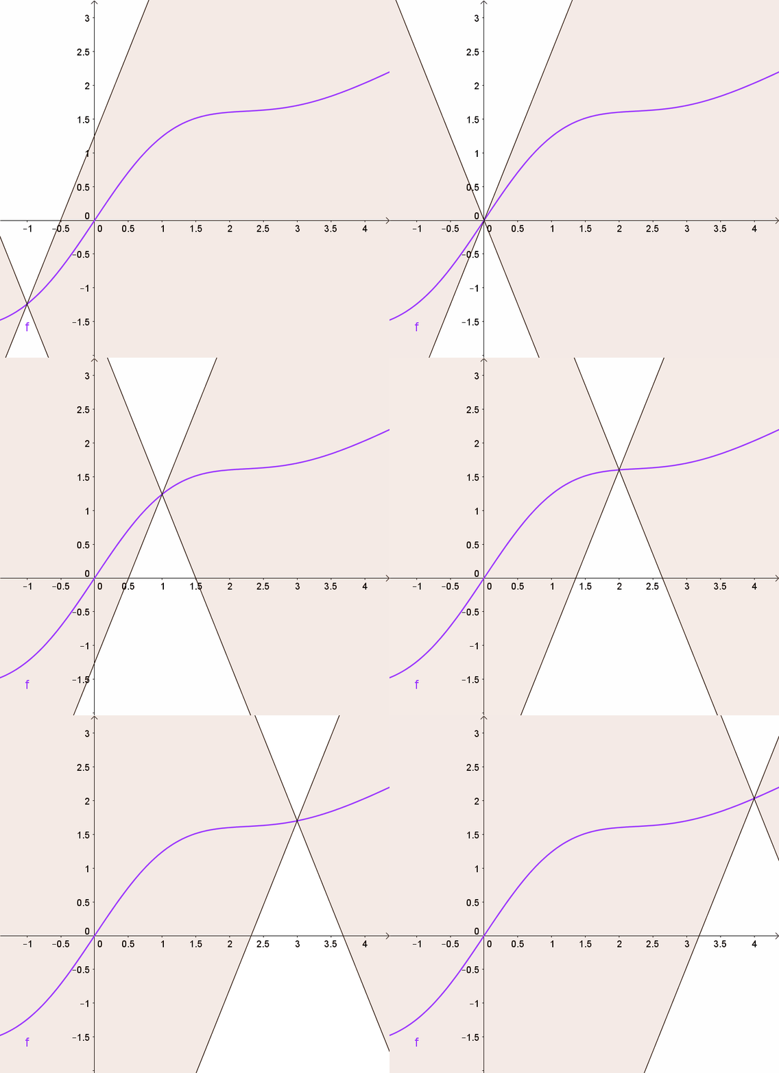
Ray Marching?
shape
A quick refresher
Lipschitz continuity
A quick refresher

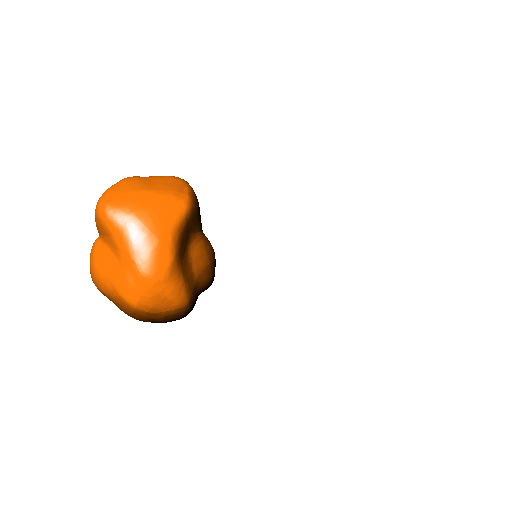
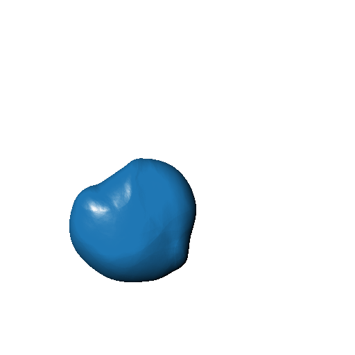
k inscribed spheres
"medial atoms"
depth
A quick refresher
"Topological Skeleton"
Medial Axis / Surface
Medial atoms are easy to regularize, and provide good multi-view priors
k inscribed spheres
"medial atoms"
A quick refresher
"Topological Skeleton"
Medial Axis / Surface
Medial atoms are easy to regularize, and provide good priors / inductive bias
k inscribed spheres
"medial atoms"
A quick refresher
"Topological Skeleton"
Medial Axis / Surface
Medial atoms are easy to regularize, and provide good priors / inductive bias
Number of candidate predictions per ray.
A quick refresher
Our Contributions
- Improve gradient flow with
probabilistic blending - Double cover the medial surface
to represent more shapes - Reduce view overfitting
- Improve how the loss is allocated
between candidate predictions - Improve the loss function itself
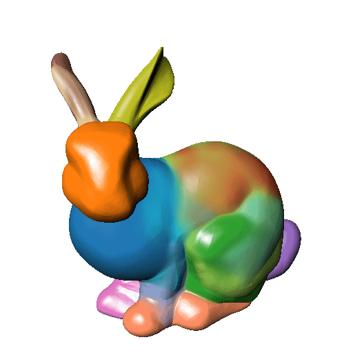
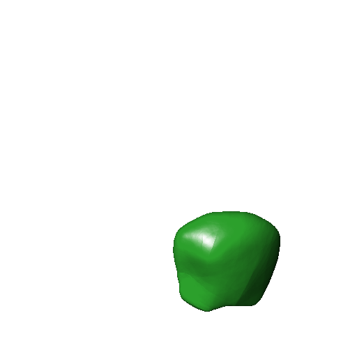
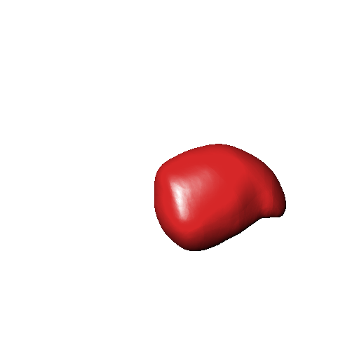
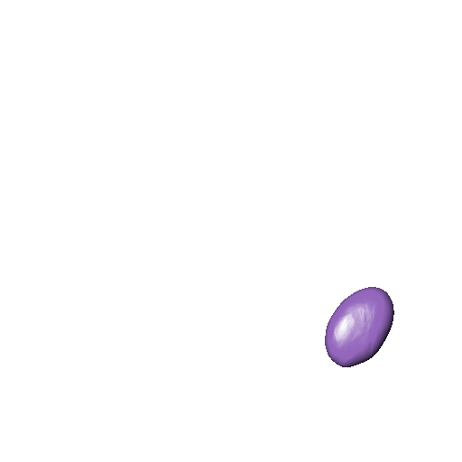
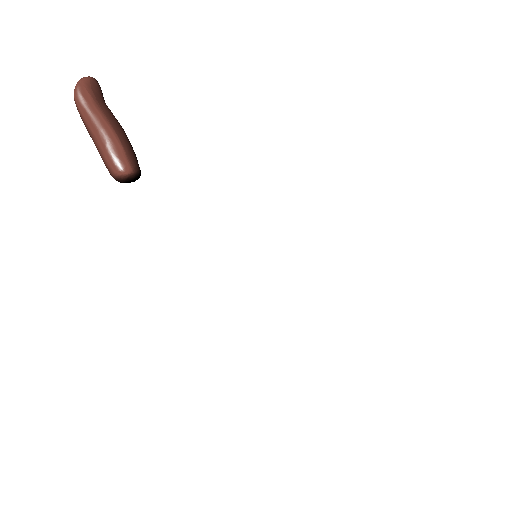
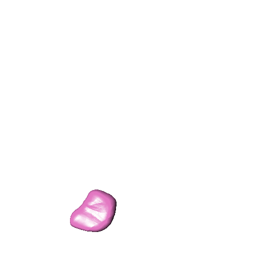
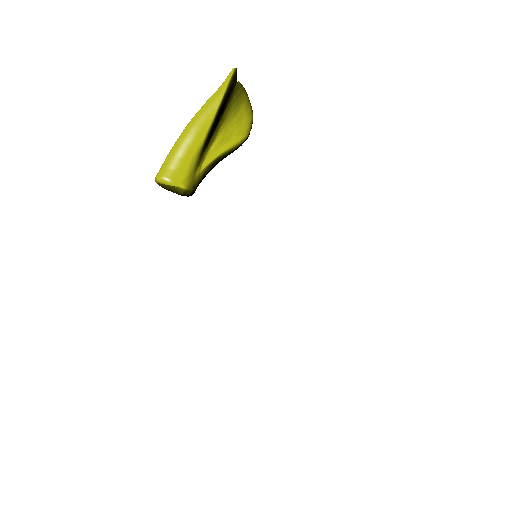
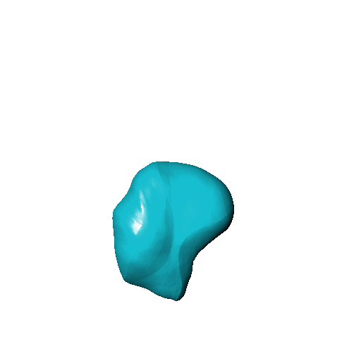
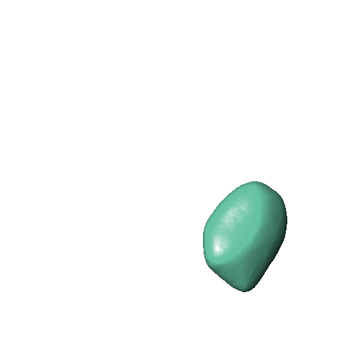
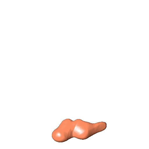
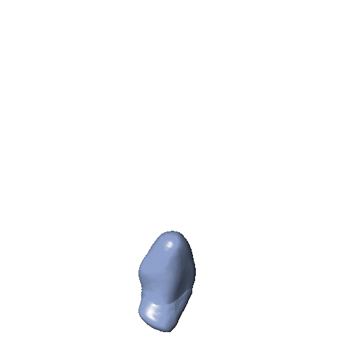
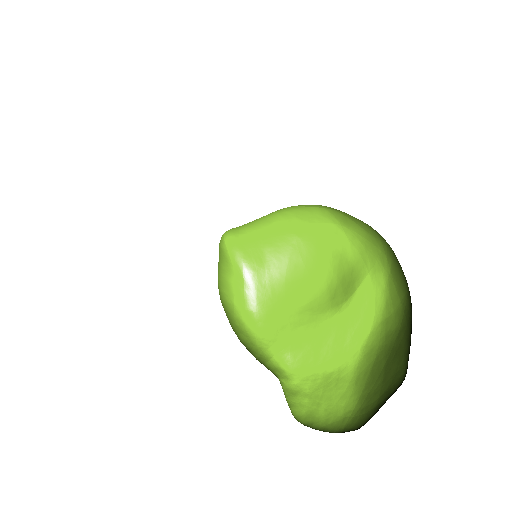
- Number of atoms predicted per ray
- Number of representable discontinuities
... but increasing k beyond 16 does not improve reconstruction quality much in practice...
Why?
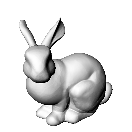
k determines:
hyperparameter
The
Atoms obscure each other
I.e. there is poor gradient flow
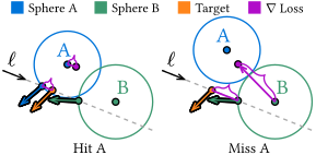
Atoms obscure each other
I.e. there is poor gradient flow
Fuzzy rendering
Why not Gaussians?
They works great for color rendering,
Towards
but not for solid surfaces.
Why not Gaussians?
Fuzzy rendering
Gaussians (or metaballs) are...
- Additive: Stacking Gaussians
cause the covered volume to grow.- Cannot use medial axis
properties for regularization
- Cannot use medial axis
- View-dependent if splatted
- Detrimental to training multi-view stability
- or require iterative ray-surface root finding
- Divergent computation, not feed-forward
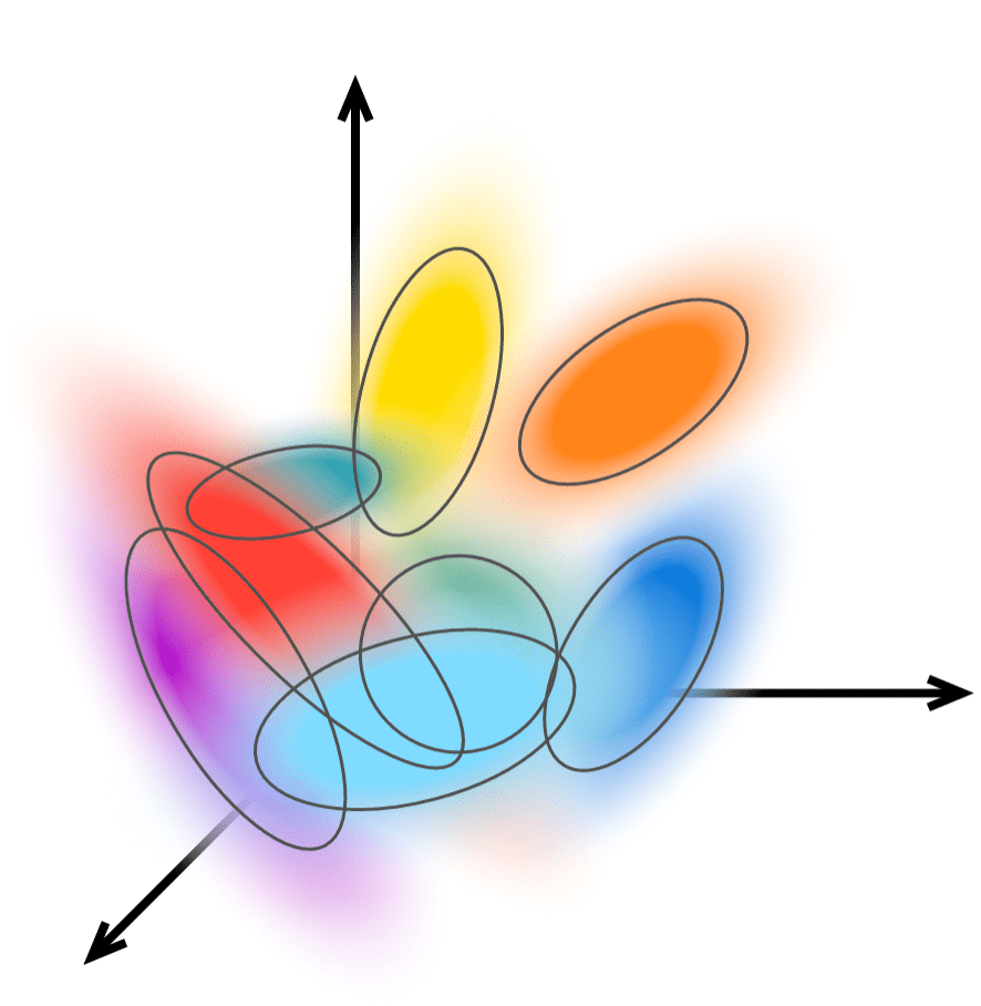
It works great for color
Towards
Fuzzy rendering
Then what?
Consider the ray-to-surface mapping

Fuzzy rendering
Then what?
Consider the ray-to-surface mapping
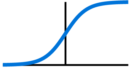
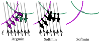
Smoothness
through erosion.
Silhouettes unaffected.
View dependent.
Figure:
Softmin atom normals
Atoms cooperate and specialize to
different parts of the shape
Atoms compete to fit the shape
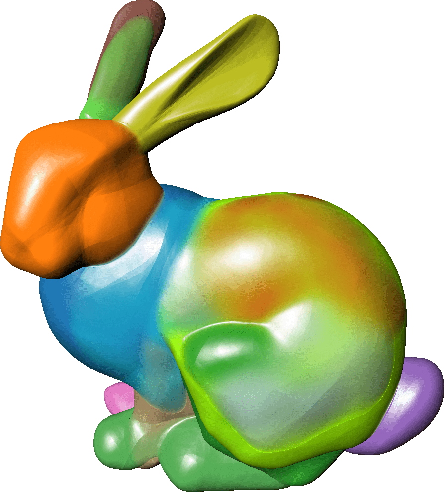
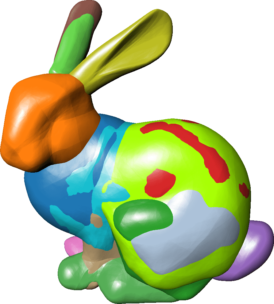
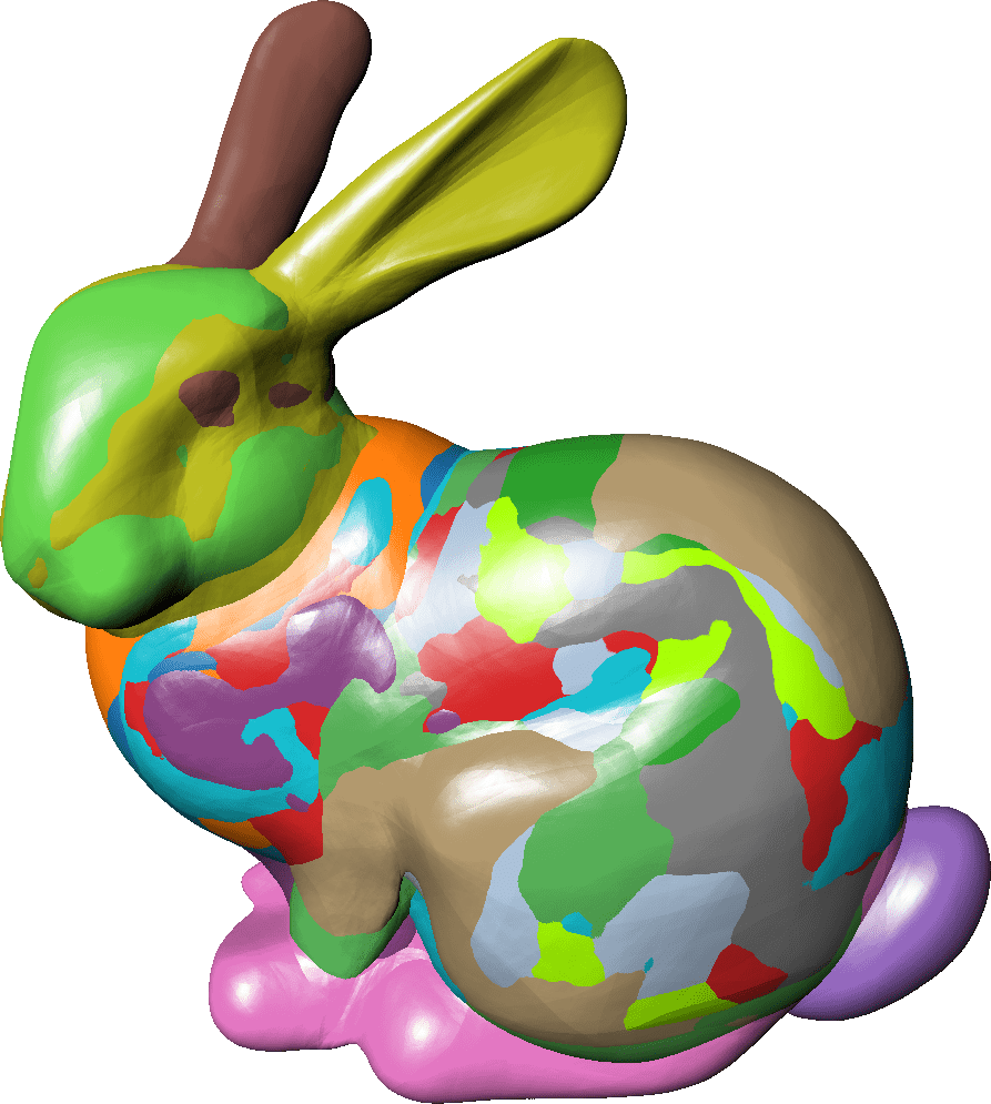
Train:
Test:
Train:
Test:
Train:
Test:
Softmin Temperature T
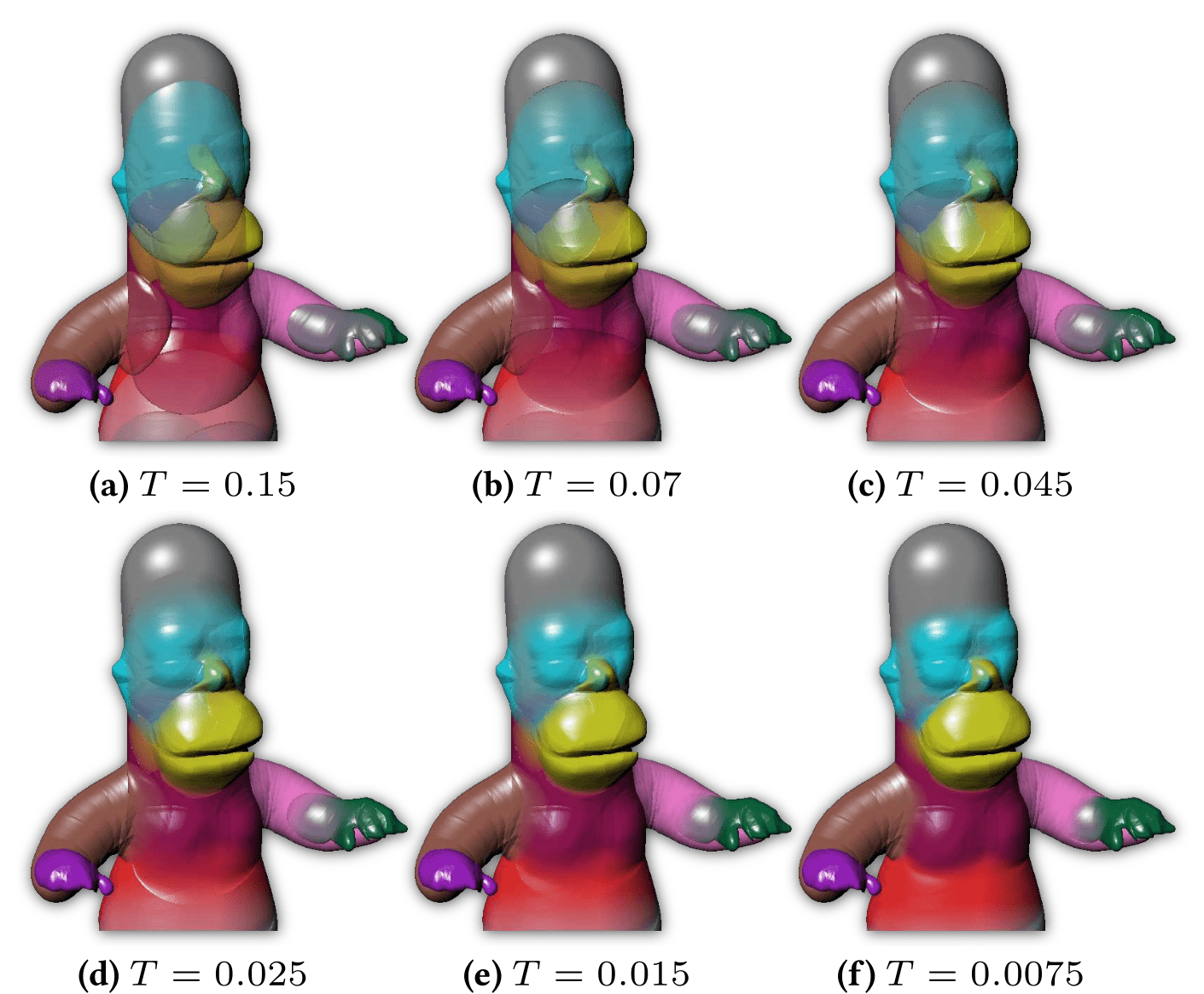
We start training at (c) then decay to (f)
Controls blending sharpness/entropy
Double-covering
The Medial Axis
First some preliminaries on parametric MARFs
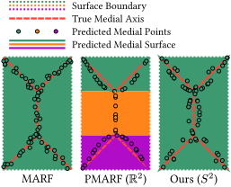
Double-covering
The Medial Axis
A ray
k atoms
Method
Double-covering
The Medial Axis
A ray
k atoms
k coordinates
Method
In essence, fit k
parametric surfaces
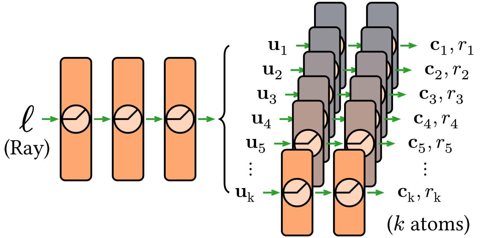
Couples the atom center and radius,
forms a consistent medial surface.
Shape is however limited
to k medial planes.
Double-covering
The Medial Axis
A ray
k atoms
k coordinates
Method
Requires a parameter-domain jump w.r.t input ray
In essence, fit k
parametric surfaces
Double-covering
The Medial Axis
A ray
k atoms
k coordinates
Method
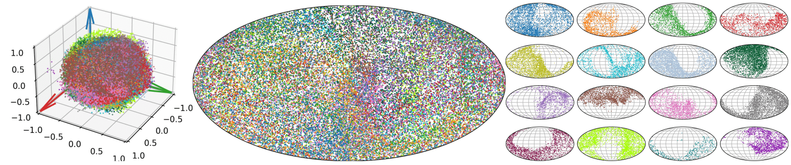
The 3D unit sphere
Double-covering
The Medial Axis
The 3D unit sphere
Double-covering
The Medial Axis
This works for any axis, provided no cycles are formed.
(i.e. on genus-0 subsets)
The 3D unit sphere
The union of two such
shapes may have any genus.
Double-covering
The Medial Axis
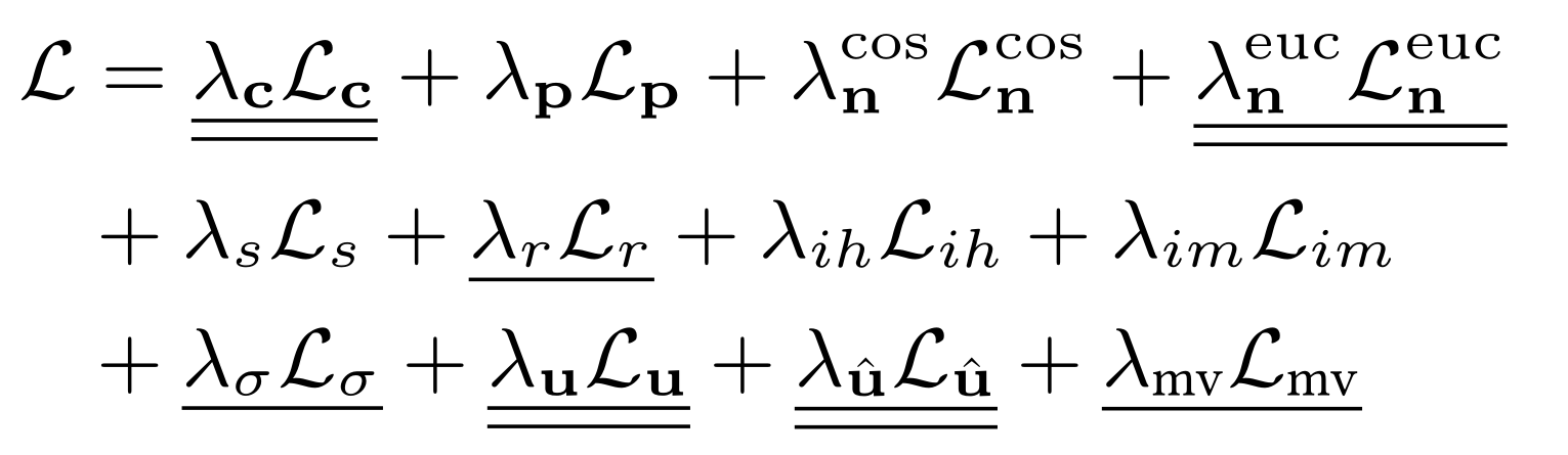
Equation: Objective Function
Constrain to unit sphere
Maximize utilization
The 3D unit sphere
Double-covering
The Medial Axis
Equation: Objective Function
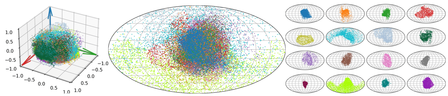
Required to leverage
wrap-around sphere topology
The 3D unit sphere
Constrain to unit sphere
Maximize utilization
Dense Data
Data Synthesis
Data Augmentation
Reducing View Overfitting
With a coarse-to-fine training schedule,
to not compromise the final fidelity.
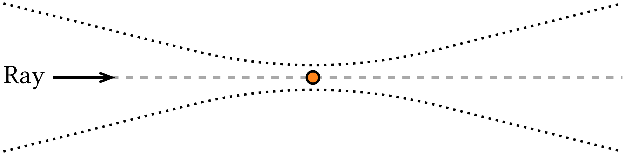
Gaussian Beam Distribution
Slope
Reducing View Overfitting
Inspired by Rebain et al. (2024) we permute rays with a
Rebain D, Yazdani S, Yi KM, Tagliasacchi A. Neural fields as distributions: Signal processing beyond Euclidean space. In 2024 IEEE/CVF Conference on Computer Vision and Pattern Recognition (CVPR) 2024 Jun 16 (pp. 4274-4283). IEEE.
Slope
Waist
Reducing View Overfitting
Gaussian Beam Distribution
Inspired by Rebain et al. (2024) we permute rays with a
Rebain D, Yazdani S, Yi KM, Tagliasacchi A. Neural fields as distributions: Signal processing beyond Euclidean space. In 2024 IEEE/CVF Conference on Computer Vision and Pattern Recognition (CVPR) 2024 Jun 16 (pp. 4274-4283). IEEE.
Slope
Waist
Rebain D, Yazdani S, Yi KM, Tagliasacchi A. Neural fields as distributions: Signal processing beyond Euclidean space. In 2024 IEEE/CVF Conference on Computer Vision and Pattern Recognition (CVPR) 2024 Jun 16 (pp. 4274-4283). IEEE.
Reducing View Overfitting
Gaussian Beam Distribution
We decay from a wide beam to
a tight beam during training.
Inspired by Rebain et al. (2024) we permute rays with a
We permute the predicted
Parameter Domain Coordinates
Reducing View Overfitting
Reducing View Overfitting
with decaying Gaussian noise
Works better when we don't
clamp the radial component
We permute the predicted
Parameter Domain Coordinates
Reducing View Overfitting
We decay the softmin blending temperature T
(sharpness/entropy)
Soft/"see through",
good gradient flow
Sharp/high fidelity,
reduced gradient flow
Reducing View Overfitting
We decay the softmin blending temperature T
(sharpness/entropy)
Reducing View Overfitting
We decay the amount of dropout from excessive to minimal,
in effect band-limiting the initial fit to avoid local minima.
Atom Selection
Improving
I.e. how the gradient is allocated between the predicted atoms.
Atom Selection
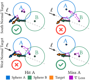
With softmin the gradient propagate to
multiple atoms, but only true hits.
Furthermore, the first hit still receive
the majority of the signal.
Improving
Furthermore, the first hit still receive
the majority of the signal.
Atom Selection
With softmin the gradient propagate to
multiple atoms, but only true hits.
Atom Selection
How?
The distance metric
Atom Selection
MARF blends atoms
using the argmin of this metric
Miss predictions are discarded
Prefers the hit furthest along negative ray direction
Supervised
(SAS)
The distance metric
Atom Selection
Supervised
Invariant of hit/miss predictions,
only the ground truth matters
This metric however requires ground truths, making it
only apply to training, not to validation or testing.
We instead prefer the atom that
has to move the least
⇒ Repair false misses,
improving recall.
⇒ View-invariant
softmin blending.
(SAS)
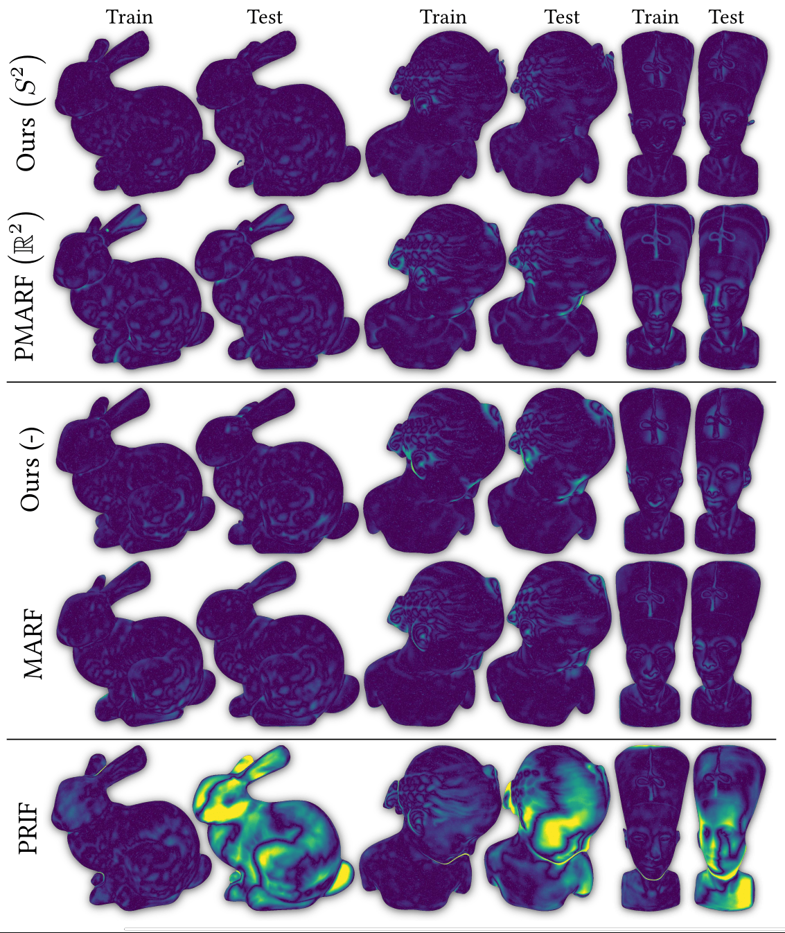
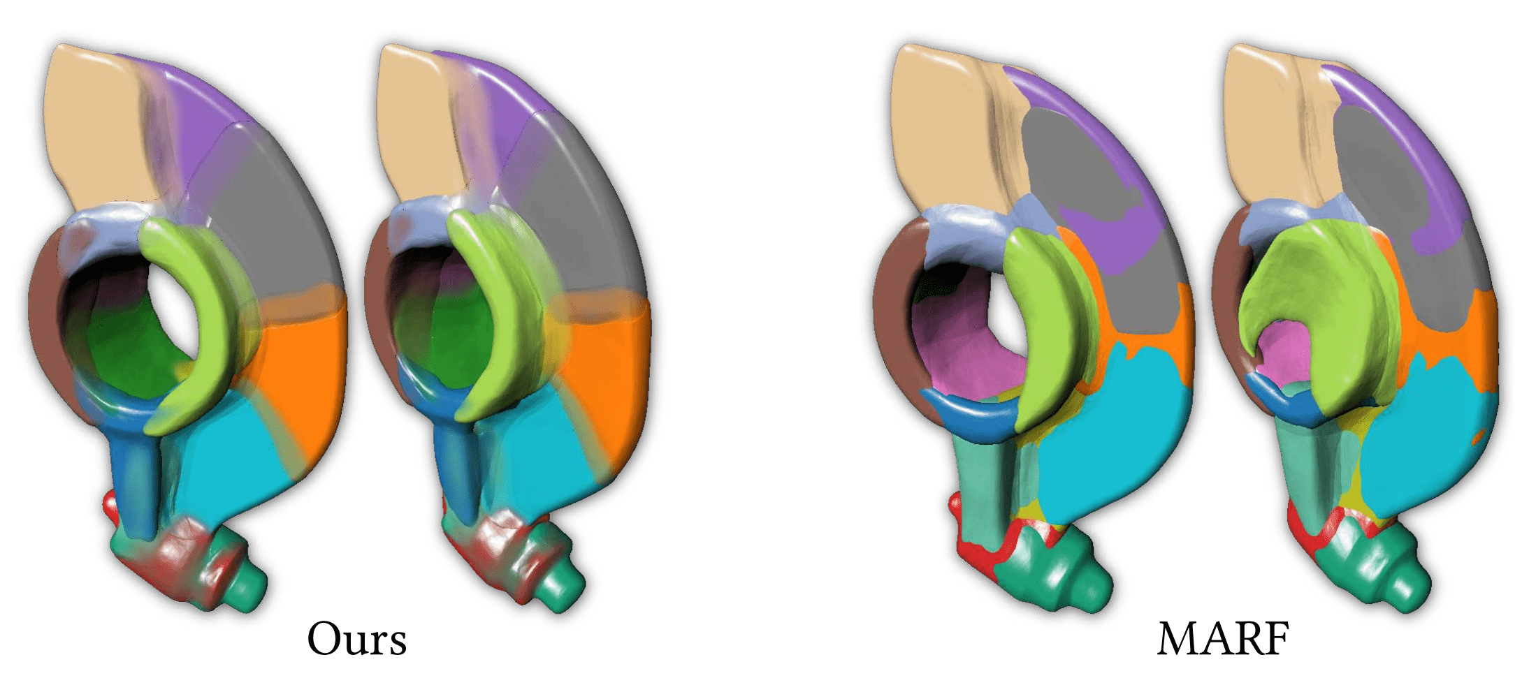
Figure:
Reconstruction error of
a training view and
a novel view, 15° apart.
Shading: Chamfer distance
to ground truth mesh.
Atom Selection
Supervised
(SAS)
Our method repairs the silhouette missed by MARF
Objective Function
The MARF loss is good for surface details,
but struggles with atom specialization,
false misses/poor recall, and has
a hit/miss imbalance.
Improving the
Atom Displacement Loss
Atom Displacement loss
Euclidean Normal Loss
Early MV loss
Truncated regularization
Parameter domain
regularization
Atom Displacement Loss
Can pull in opposite directions!
Applies to true hits only
Objective Function
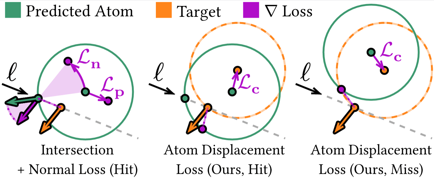
Pushes atom along ray
to fit target depth
Pivots atom about hit
to fit target surface normal
Atom Displacement Loss
Recall our SAS:
Prefers the atom that
has to move the least.
What if we penalize
this distance?
Objective Function
Atom Displacement Loss
Applies to all hits
Supervises intersection points
and normals jointly
Objective Function
Atom Displacement Loss
Euclidean Normal loss
Objective Function
Euclidean Normal loss
Atom Displacement Loss
Early Multi-View
Objective Function
Euclidean Normal loss
Atom Displacement Loss
Early Multi-View
Cosine Distance
Euclidean Distance

Yin R, Chen Y, Karaoglu S, Gevers T. Ray-Distance Volume Rendering for Neural Scene Reconstruction. In: Leonardis A, Ricci E, Roth S, Russakovsky O, Sattler T, Varol G, editors. Computer Vision – ECCV 2024, Cham: Springer Nature Switzerland; 2025, p. 377–94.
https://doi.org/10.1007/978-3-031-72630-9_22
Smooth and stable
Sharp, but unstable
Objective Function
Normal loss
Early Multi-View
First, a small recap
Double backpropagation
Objective Function
Early Multi-View
... how does differentiating w.r.t. the ray direction help?
Ray
Hit
Objective Function
Early Multi-View
Ray
Hit
4D embedding
Global along-ray translation invariance
by construction through normalization
or
Ray origin is normalized
before network ever sees it,
but is still a part of the
auto-differentiation graph!
Objective Function
Early Multi-View
Ray
Hit
4D embedding
or
penalizing changes w.r.t. viewpoint.
Objective Function
Early Multi-View
Global along-ray translation invariance
by construction through normalization
Ray origin is normalized
before network ever sees it,
but is still a part of the
auto-differentiation graph!
Objective Function
Early Multi-View
Fix intersected atom center and radius, not just the intersection point.
Objective Function
Early Multi-View
Ray Decoder
Wastes capacity to accommodate
a multi-view inconsistent ray decoder
Objective Function
Early Multi-View
Medial Surface Decoders
- Skip lots of double backprop
- Multi-view consistent
ray decoder
Weighted with softmin weights
Objective Function
Early Multi-View
Truncated Regularization
Objective Function
Truncated Regularization
Early Multi-View
A brief recap
Objective Function
Truncated Regularization
Early Multi-View
adds a constant positive pressure on atom radii (MAT maximality).
limits per-candidate area of influence, to specialize atoms to separate parts and handle discontinuities.
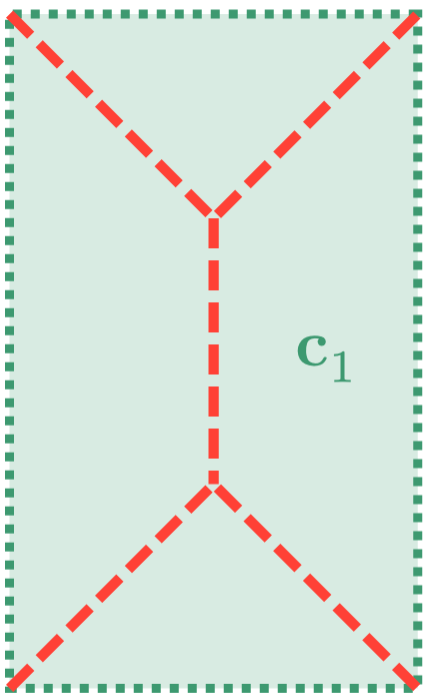
there is a single trivial solution
when no other loss apply.
Failure mode:
Objective Function
Truncated Regularization
Early Multi-View
adds a constant positive pressure on atom radii (MAT maximality).
limits per-candidate area of influence, to specialize atoms to separate parts and handle discontinuities.
there is a single trivial solution
when no other loss apply.
Failure mode:
The majority of predictions miss,
from a per-candidate perspective.
Objective Function
Truncated Regularization
Early Multi-View
adds a constant positive pressure on atom radii (MAT maximality).
limits per-candidate area of influence, to specialize atoms to separate parts and handle discontinuities.
there is a single trivial solution
when no other loss apply.
Failure mode:
The majority of predictions miss,
from a per-candidate perspective.
- Reconstruction quality
- Scaling behavior
- Ablations studies
- Training and
rendering speed
3 architectures
2 setups
( + PRIF )
Results
Results
Reconstruction
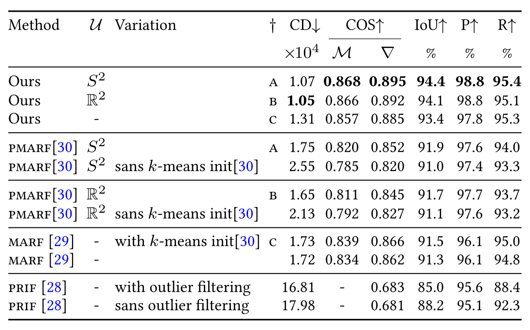
Table: Reconstruction scores. Average of 19 shapes.
Results
Reconstruction
Table: Reconstruction scores. Average of 19 shapes.
Depth-based
(non-medial)
Medial baselines
Baseline
with our S²
Our softmin & improved loss
Chamfer Distance
Cosine Similarity
Medial Atom Normals
Differential Normals
Intersection over Union
Precision
Recall
Results
Reconstruction
Table: Reconstruction scores. Average of 19 shapes.
Results
Reconstruction
Table: Reconstruction scores. Average of 19 shapes.
Results
Reconstruction
Table: Reconstruction scores. Average of 19 shapes.
Results
Reconstruction
Table: Reconstruction scores. Average of 19 shapes.
Results
Reconstruction
Table: Reconstruction scores. Average of 19 shapes.
Results
Reconstruction
Table: Reconstruction scores. Average of 19 shapes.
Results
Reconstruction
Table: Reconstruction scores. Average of 19 shapes.
Results
Reconstruction
Table: Reconstruction scores. Average of 19 shapes.
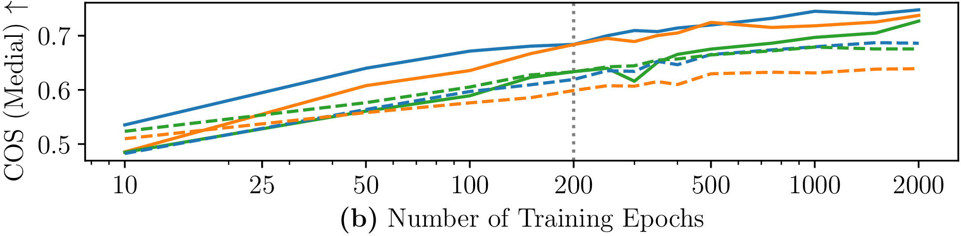
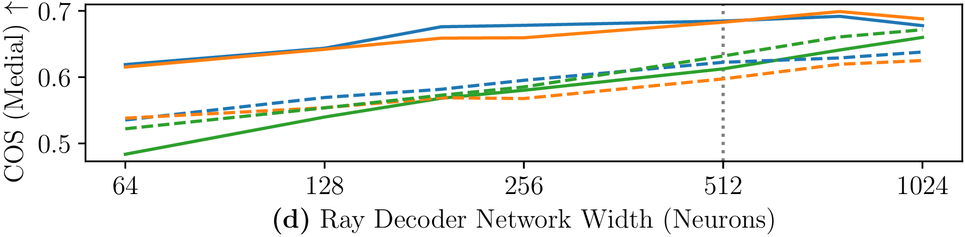
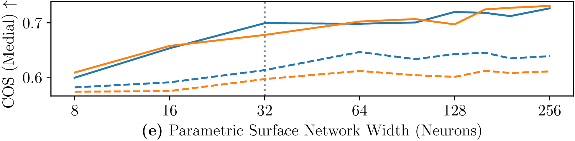
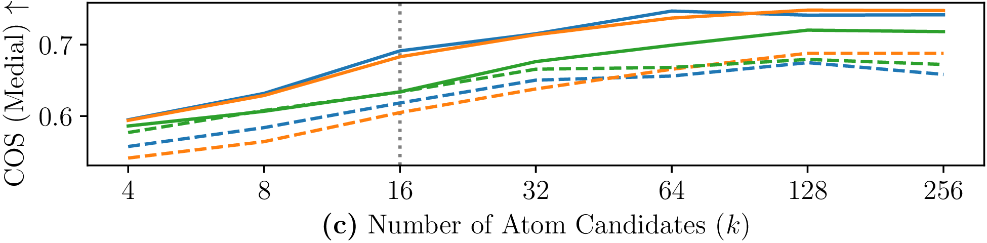
Scaling
Same correctness, with improved capacity and recall.
Best overall.
Start to fall behind.
Has a "indecisive"
fit from the higher gradient flow.
Results
Reconstruction
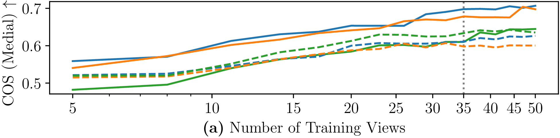

Scaling
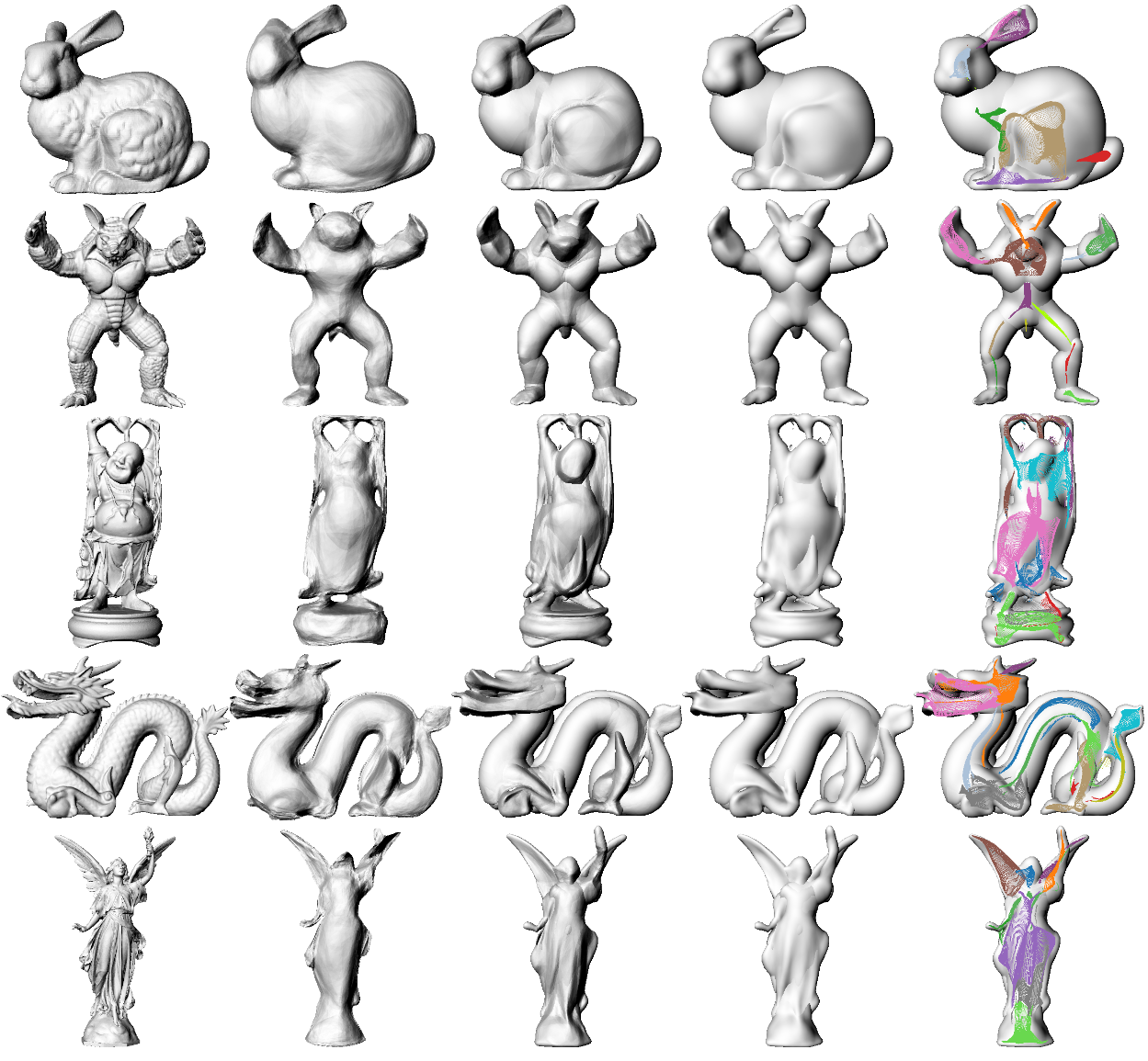
Renders
Results
Scaling
Renders
fails to generalize
multi-view stable
multi-view stable
multi-view stable
multi-view stable
multi-view stable
degeneracies near
overhangs
degeneracies near
overhangs
limited topology
limited topology
Results
Scaling
Renders
fails to generalize
multi-view stable
multi-view stable
multi-view stable
multi-view stable
multi-view stable
degeneracies near
overhangs
degeneracies near
overhangs
missing silhouette
missing silhouette
missing silhouette
limited topology
limited topology
Results
Scaling
Renders
fails to generalize
multi-view stable
multi-view stable
multi-view stable
multi-view stable
multi-view stable
degeneracies near
overhangs
degeneracies near
overhangs
missing silhouette
missing silhouette
missing silhouette
limited topology
limited topology
problems with inorganic shapes
that feature sharp angles
Renders
Reconstruction
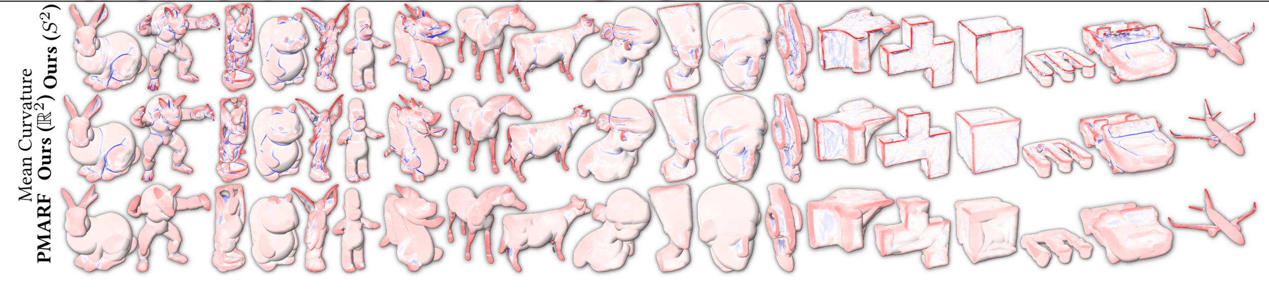
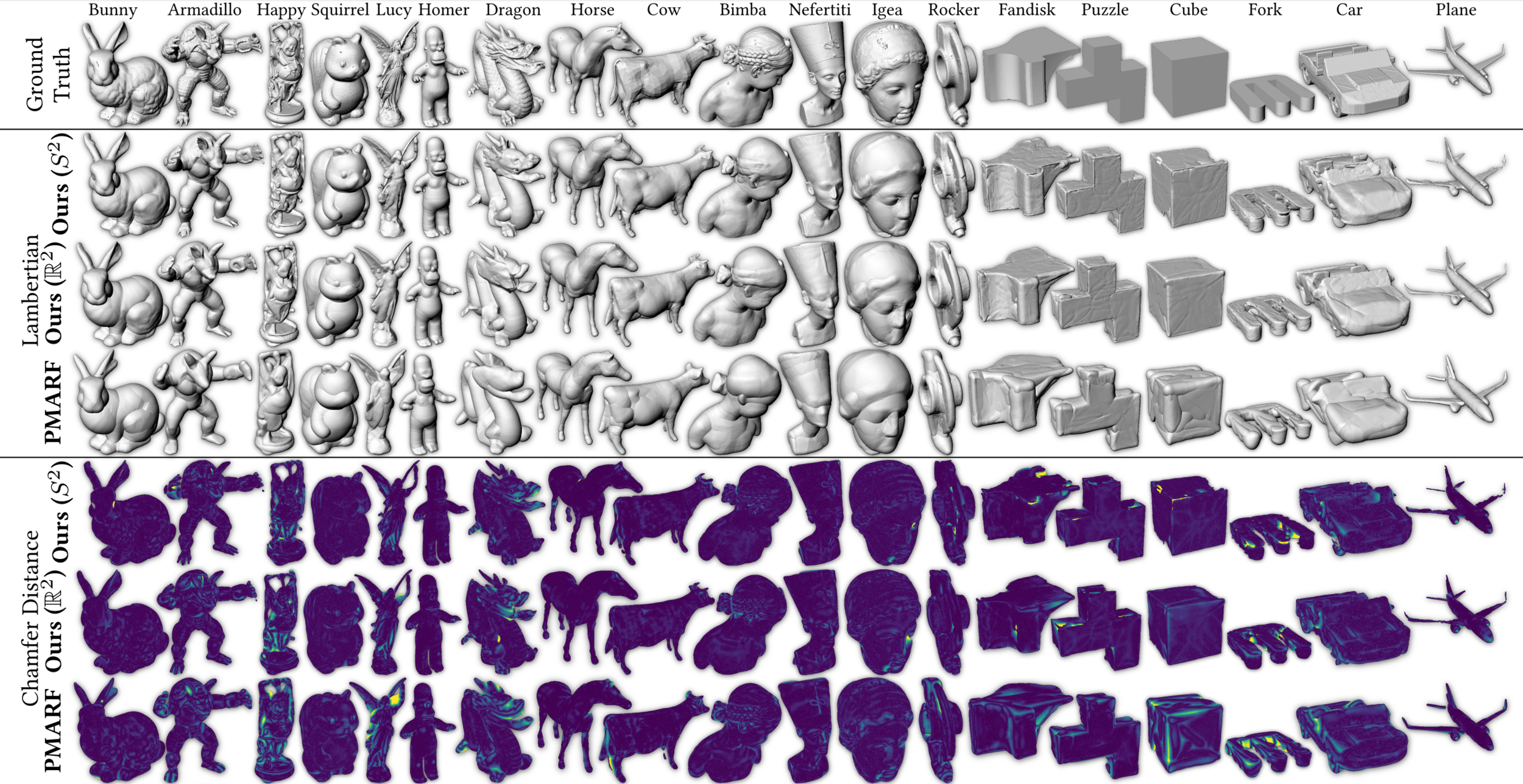
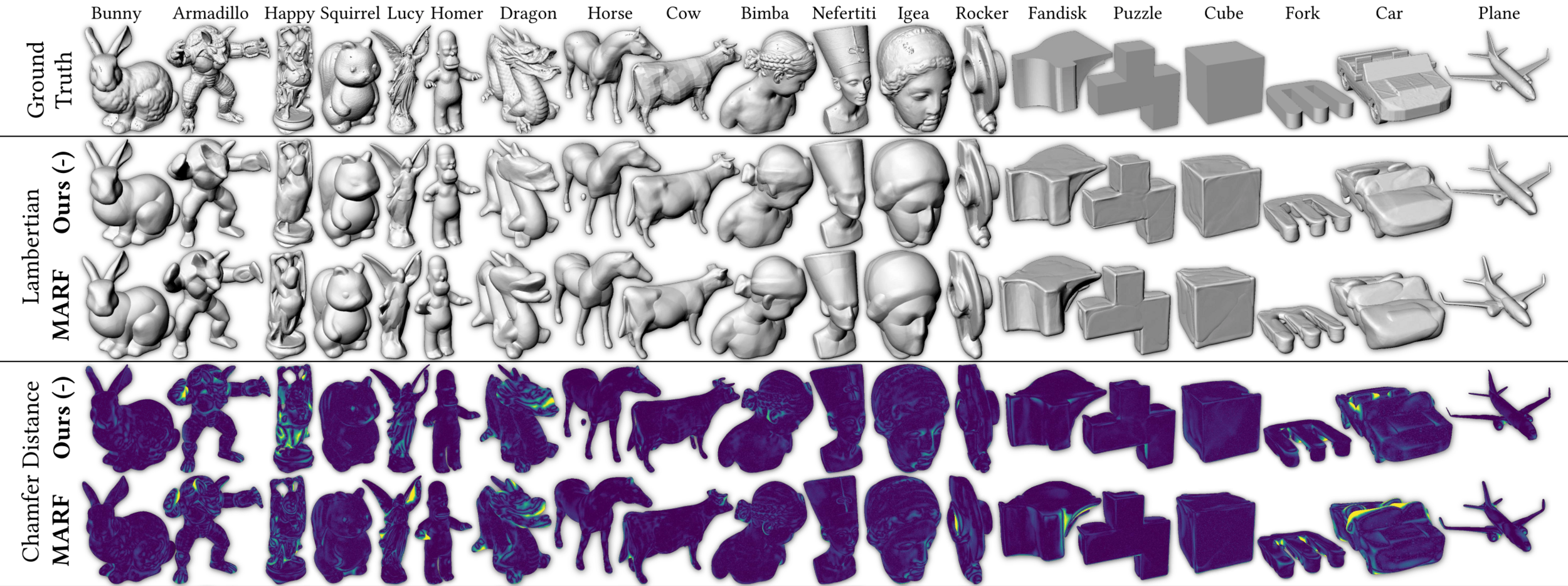

Results
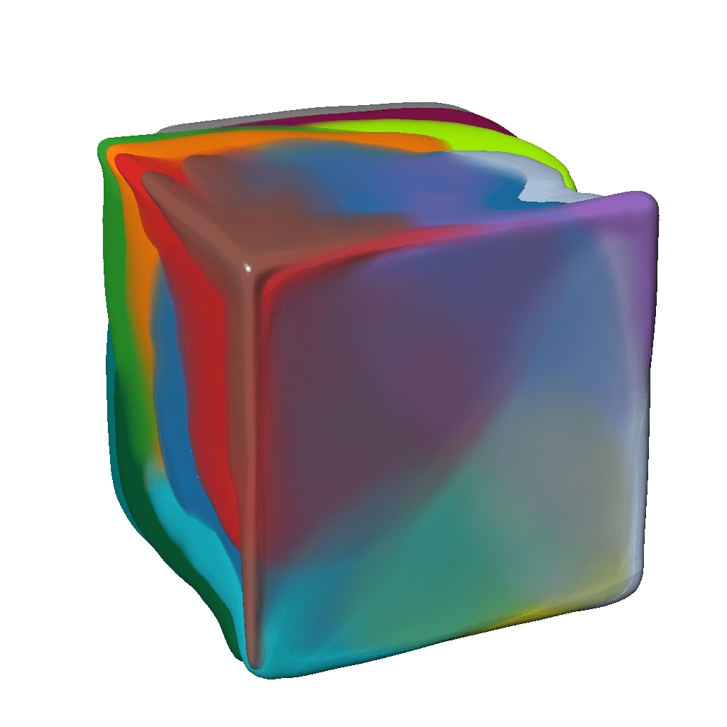
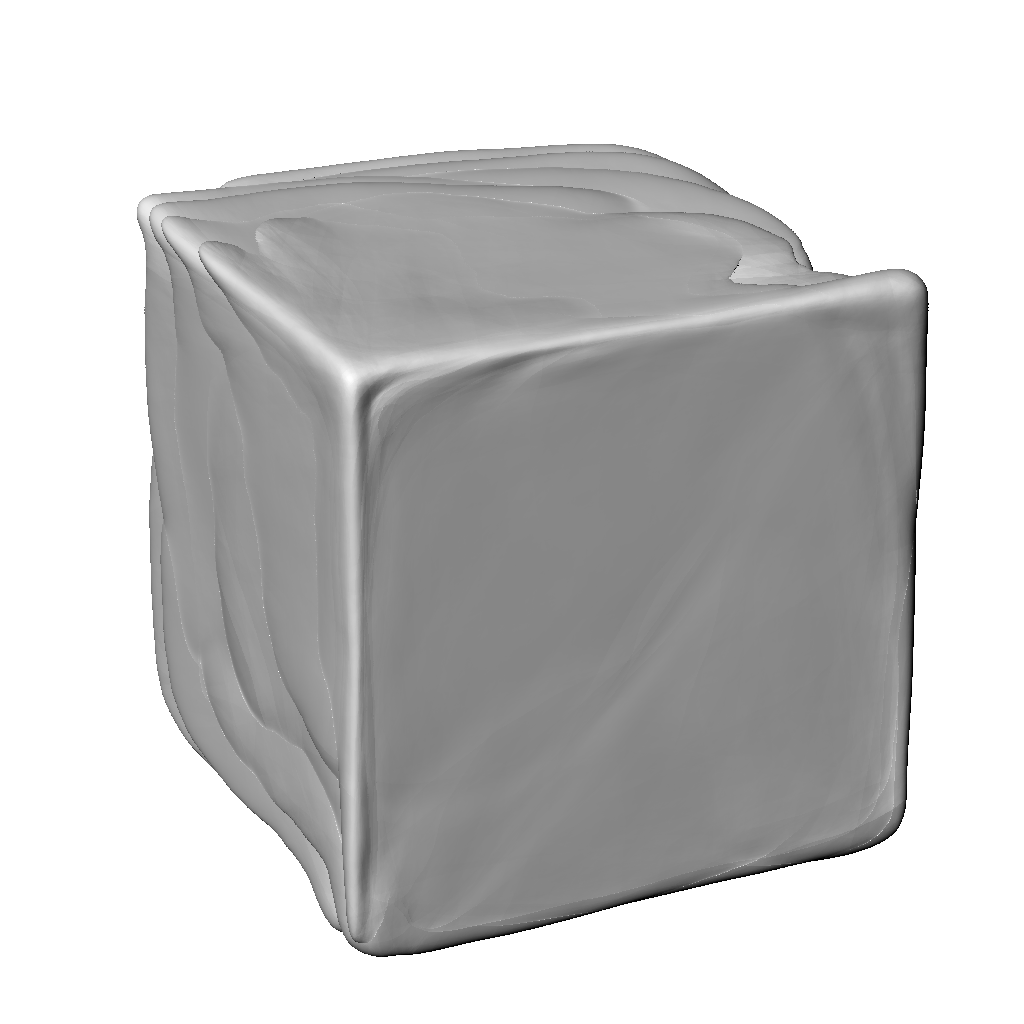
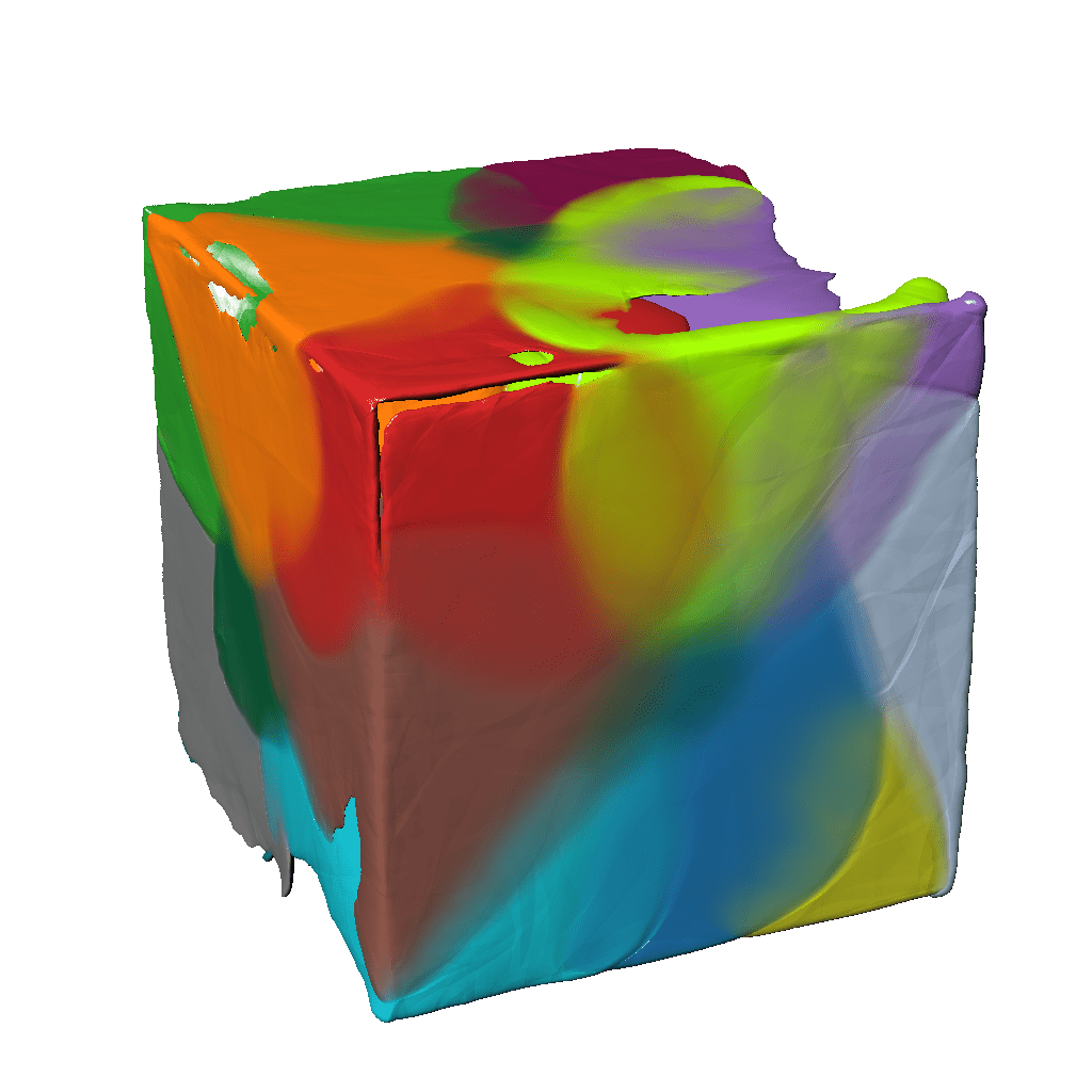
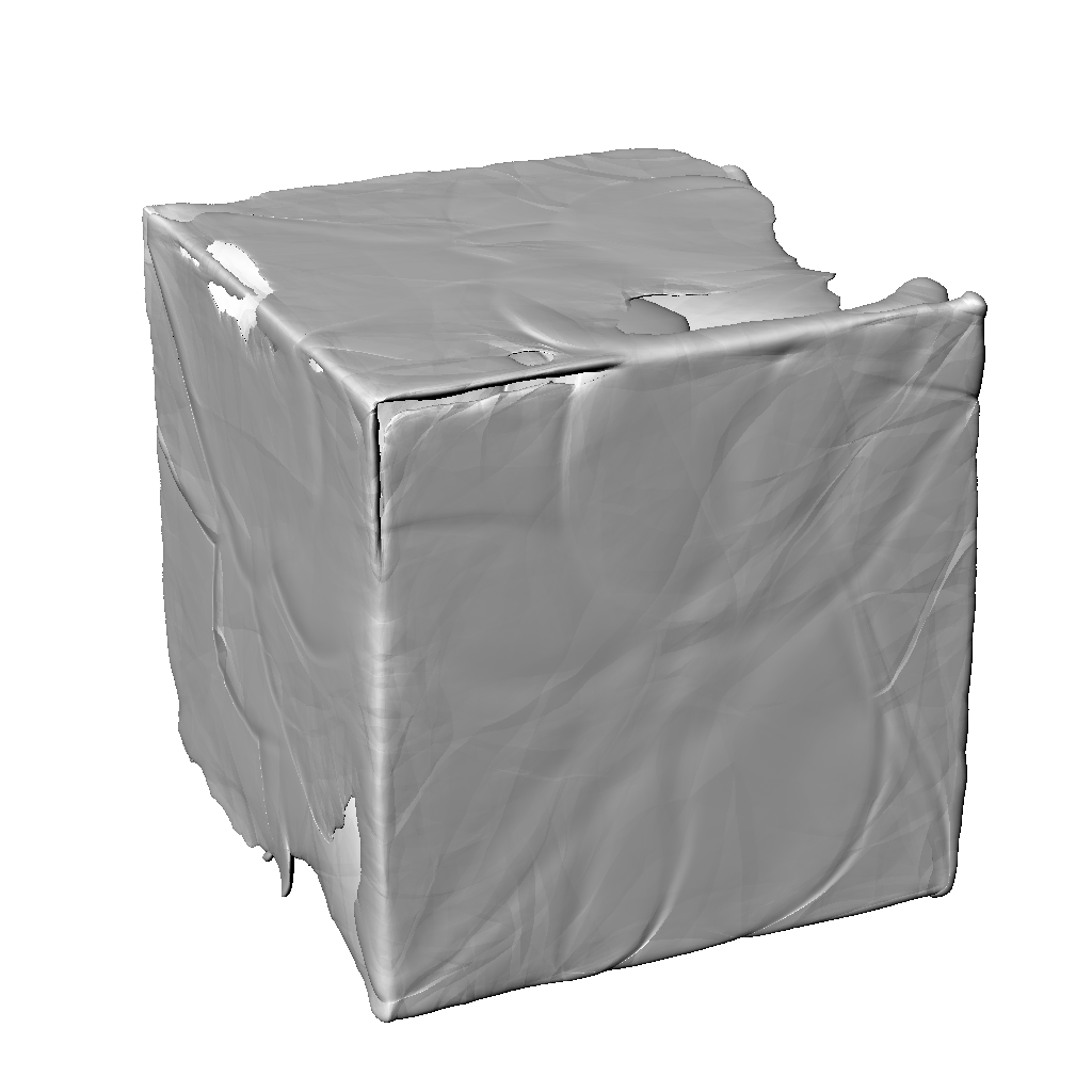
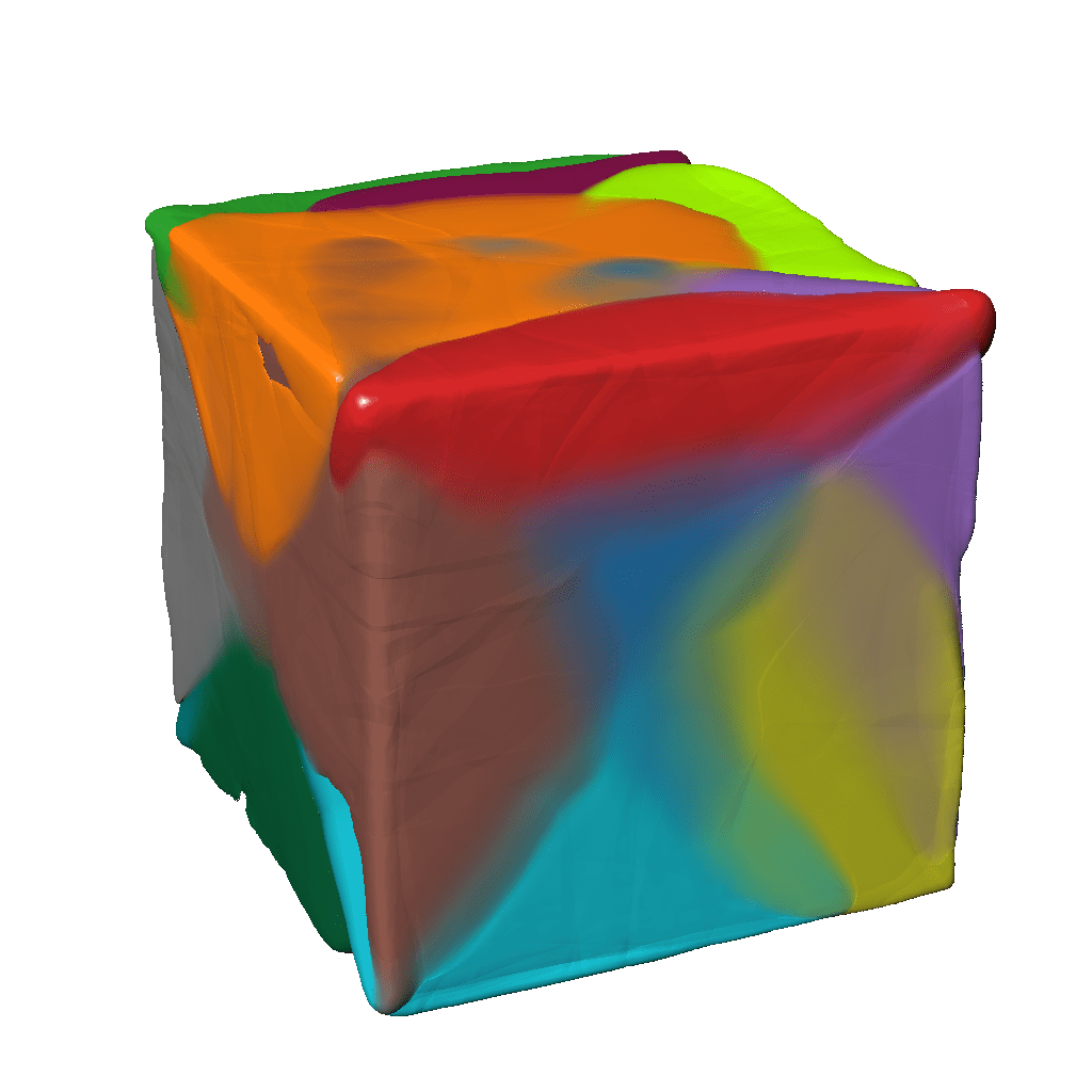
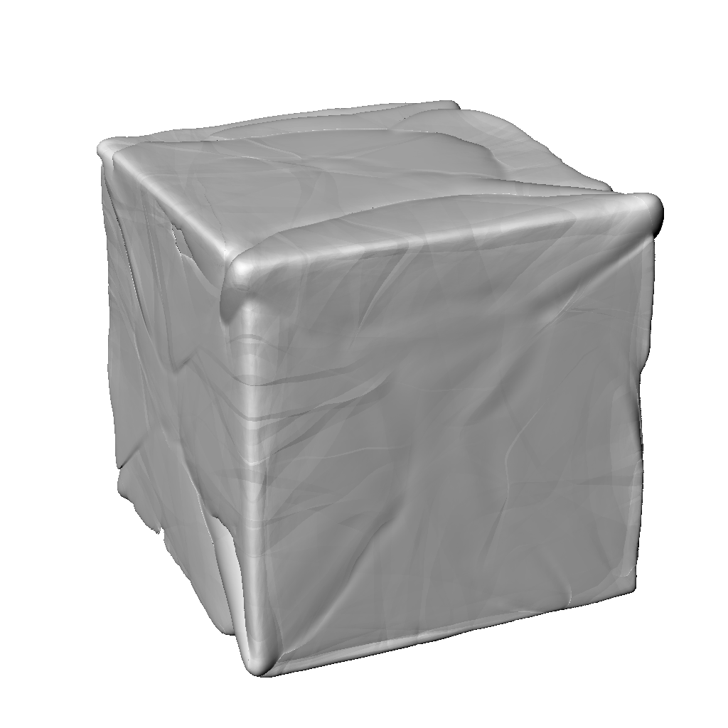
Reconstruction
Specialized
Specialized
Entangled atoms
Limited topology
Vanishing radius
Results
Reconstruction
Specialized
Specialized
Limited topology
Vanishing radius
A novel-view problem,
training views are unaffected.
Likely a ray-decoder interpolation issue.
This hurdle may be fixed with:
Rebain D, Yazdani S, Yi KM, Tagliasacchi A. Neural fields as distributions: Signal processing beyond Euclidean space. In 2024 IEEE/CVF Conference on Computer Vision and Pattern Recognition (CVPR) 2024 Jun 16 (pp. 4274-4283). IEEE.
Entangled atoms
Results
Ablations
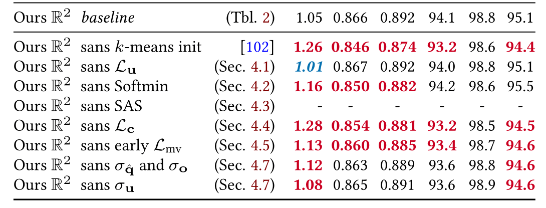
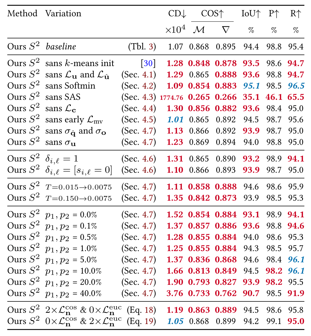
Table: Ablation studies
Table: Ablation studies
Results
Ablations
Table: Ablation studies
Table: Ablation studies
Results
Ablations
Table: Ablation studies
Table: Ablation studies
Sundt PB, Theoharis T. Towards multi-view consistency in neural ray fields using parametric medial surfaces. Computers & Graphics 2024;123:103991.
k-means init
Agnostic init
Data
Results
Ablations
Table: Ablation studies
Table: Ablation studies
but is benefitial on PMARF baselines.
Reinforces characteristics observed earlier.
Detrimental on Our R² configuration,
Results
Ablations
Table: Ablation studies
Table: Ablation studies
argmin
softmin
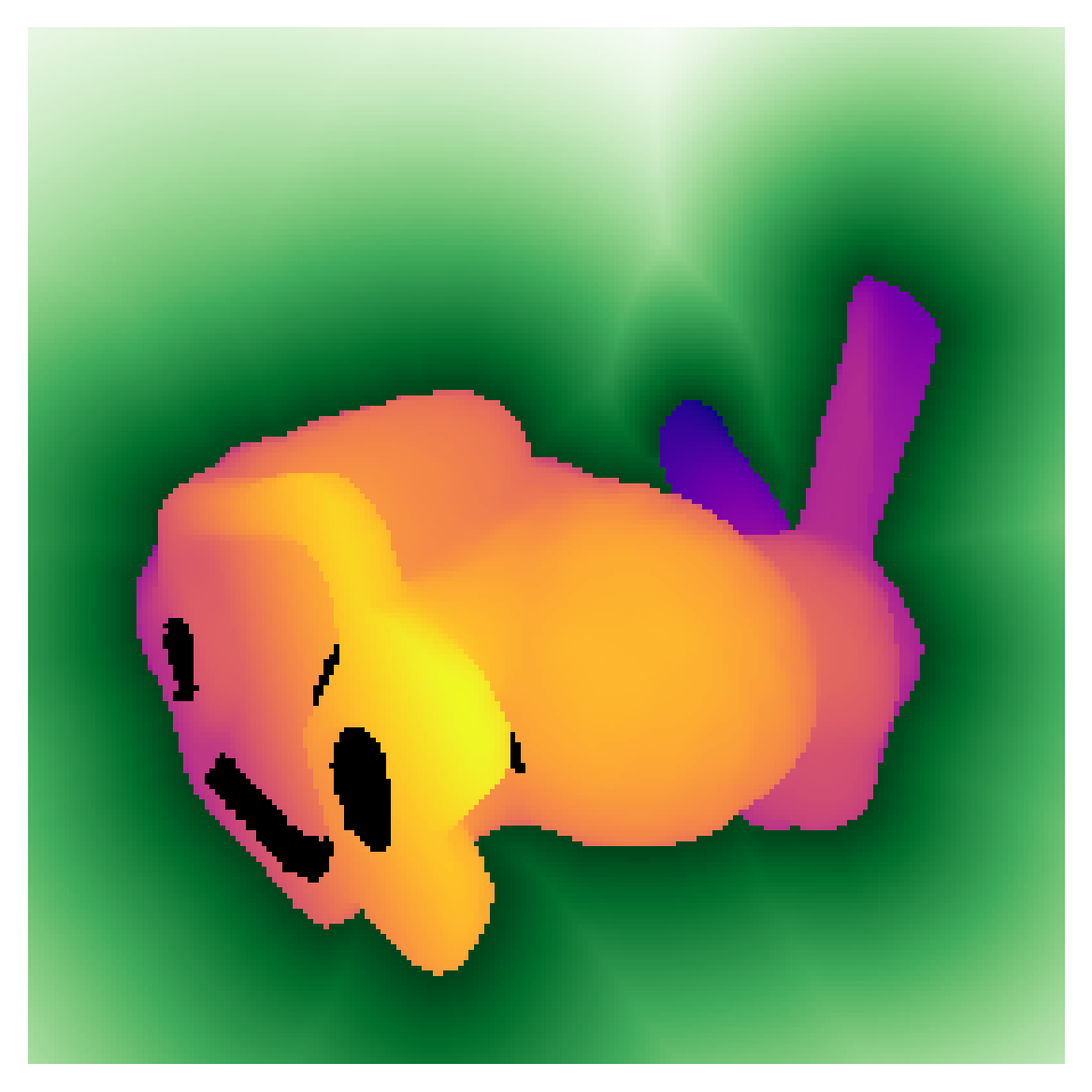
data
Results
Ablations
Table: Ablation studies
Table: Ablation studies
⇒ Our Atom Displacement Loss requires Supervised Atom Selection.
our SAS mitigates the issue.
Penalizing normals early is unstable (MARF baseline also avoids it),
Results
Ablations
Table: Ablation studies
Table: Ablation studies
Results
Ablations
Table: Ablation studies
Table: Ablation studies
Results
Ablations
Table: Ablation studies
Table: Ablation studies
Results
Ablations
Table: Ablation studies
Table: Ablation studies
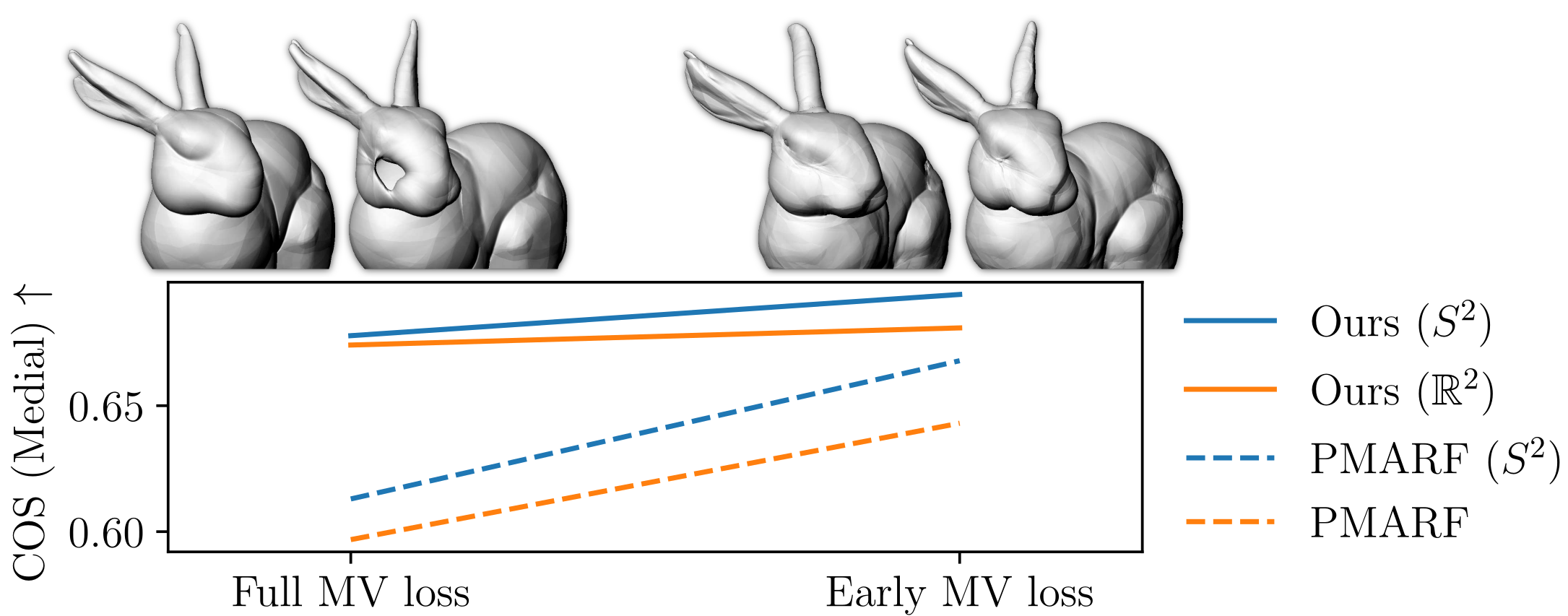
Strictly improved
Detrimental?
Primarily on mechanical shapes
Results
Ablations
Table: Ablation studies
Table: Ablation studies
Ray augmentation improves fidelity and recall.
And so does parameter domain augmentation.
Results
Ablations
Table: Ablation studies
Table: Ablation studies
And so does parameter domain augmentation.
Ray augmentation improves fidelity and recall.
Results
Ablations
Table: Ablation studies
Like MARF baseline
Hits only
Table: Ablation studies
Our 0.3 threshold strikes a sweetspot between regularizing all rays or regularizing hits only
Results
Ablations
Table: Ablation studies
Results
Ablations
Table: Ablation studies
Results
Ablations
Table: Ablation studies
Results
Ablations
Table: Ablation studies
Excessive
Insufficient
Sweetspot?
Decaying dropout
Fixed dropout
Our decay from excessive to minimal avoids
local minima without sacrificing fidelity,
but rather improve it.
Results
Ablations
Table: Ablation studies
Cosine and Euclidean
Euclidean-only
Cosine-only
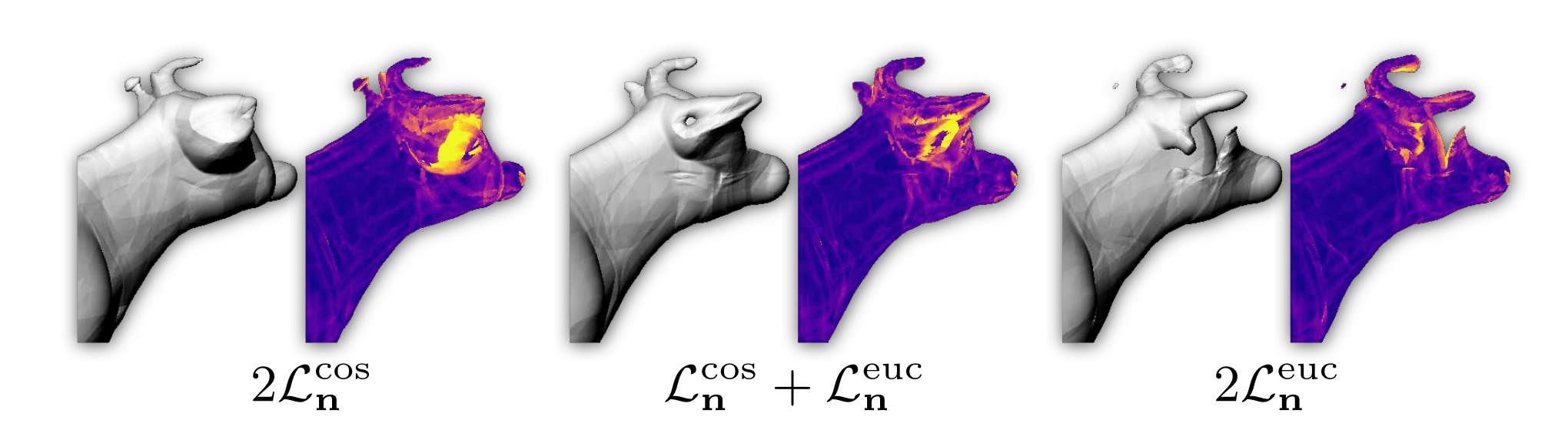
Stable, but smooth
Detailed, but unstable
A balance
Results
Runtime
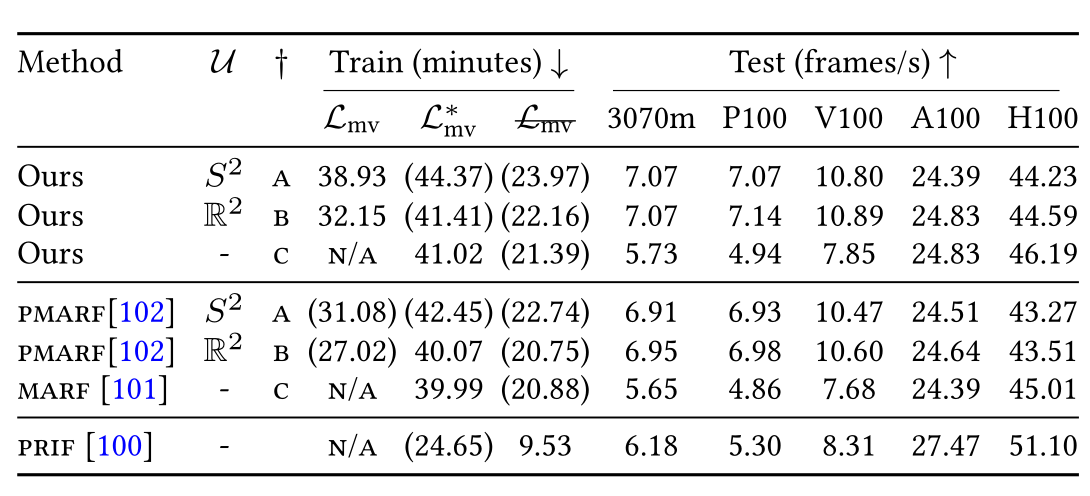
Table: Timing Results
Ours have more losses, more gradients.
S² has k more activations and a vector normalization.
Results
Runtime
Table: Timing Results
Performance is reclaimed by our early multi-view loss.
Ours have more losses, more gradients.
S² has k more activations and a vector normalization.
Results
Runtime
Table: Timing Results
Parametric networks excel when compute bound.
Softmin blending is less divergent than Argmin lookups.
Results
Runtime
Table: Timing Results
Large but simple MLPs win out when not compute bound.
Parametric networks excel when compute bound.
Softmin blending is less divergent than Argmin lookups.
Thanks
-
A new double-covering parametrization
-
Expands representation capacity
-
-
Probabilistic blending
-
Improves gradient flow and scaling
-
-
New loss functions
-
Increases fidelity, stability and recall
-
-
Faster and improved multi-view stabilization
-
Reduce training times while improving multi-view stability
-
-
Coarse-to-fine training schedule
-
Improves convergence and multi-view generalization
-