Collinson and Ganong (2018)
The economics of Housing & Homelessness
How would you frame this paper?
What mechanism would you like to have seen explored further?
What is an alternative identification strategy?
What would scaling this experiment look like?
Standard Discussion Questions
THe Essence of the Paper
The Research Question is Clear and Well Motivated
The conclusions that we're meant to take away from the paper are Clear and Precise
Overview
The underlying story though is missing...
Motivation
"Most housing voucher holders opt to live in neighborhoods of much lower quality than the average neighborhood, and typically live in neighborhoods similar to their neighborhood before receiving a voucher"
"A central goal of US low-income housing programs in recent years has been to improve neighborhood quality for assisted households"
Research Question
Motivation
What is a cost effective way to improve neighborhood quality for Section-8 vouchers?
Do the Results Make Sense?
(Or do they contradict each other)
A policy that makes vouchers more generous across a metro area benefits landlords through increased rents, with minimal impact on neighborhood and unit quality
Result # 1
A second policy that indexes rent ceilings to neighborhood rents leads voucher holders to move into higher quality neighborhoods with lower crime, poverty, and unemployment
Result # 2
Background
Voucher Background
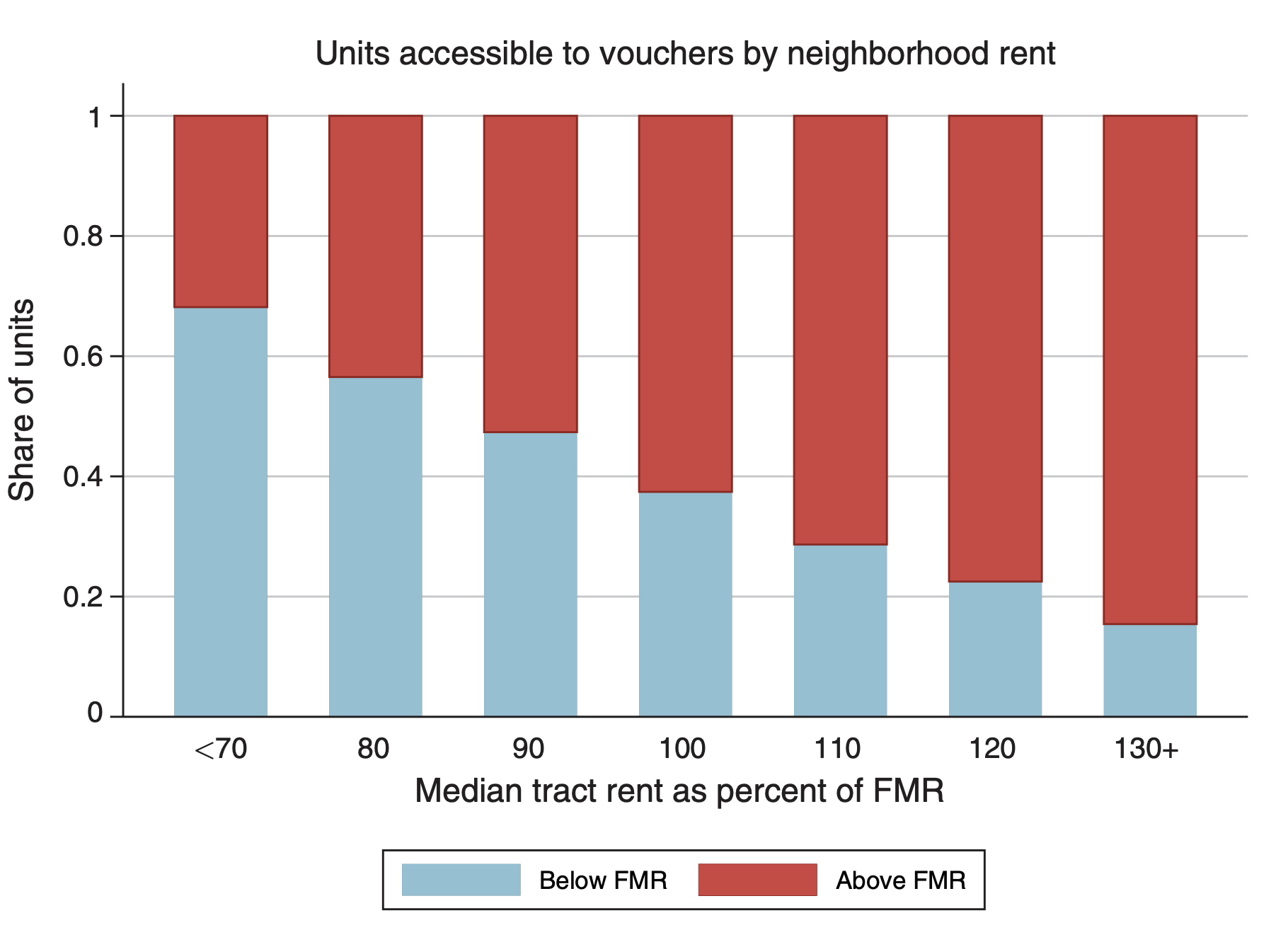
Voucher holders by 30% of their income up to a rent ceiling (fair market rent)
Rent Ceilings generally vary at the county level, but is often the same across counties within a metro area
If the unit is priced below the fair market rent, then the local housing authority (not the tenant) bears the full cost of a rent increase
Uniform Rent Increases
Uniform Rent Ceiling Increase

Description
Result
Increase the Fair Market Rent Thresholds
Rent
Neighborhood Quality
Gold Standard
Randomize Rent Ceilings Across Housing Authorities
Approach
"Find" Quasi-exogenous variation in something that effects Rent Ceilings, but doesn't affect outcomes of interest (Rental Price, Quality, and Neighborhood)
Uniform Rent Increases (Method 1)
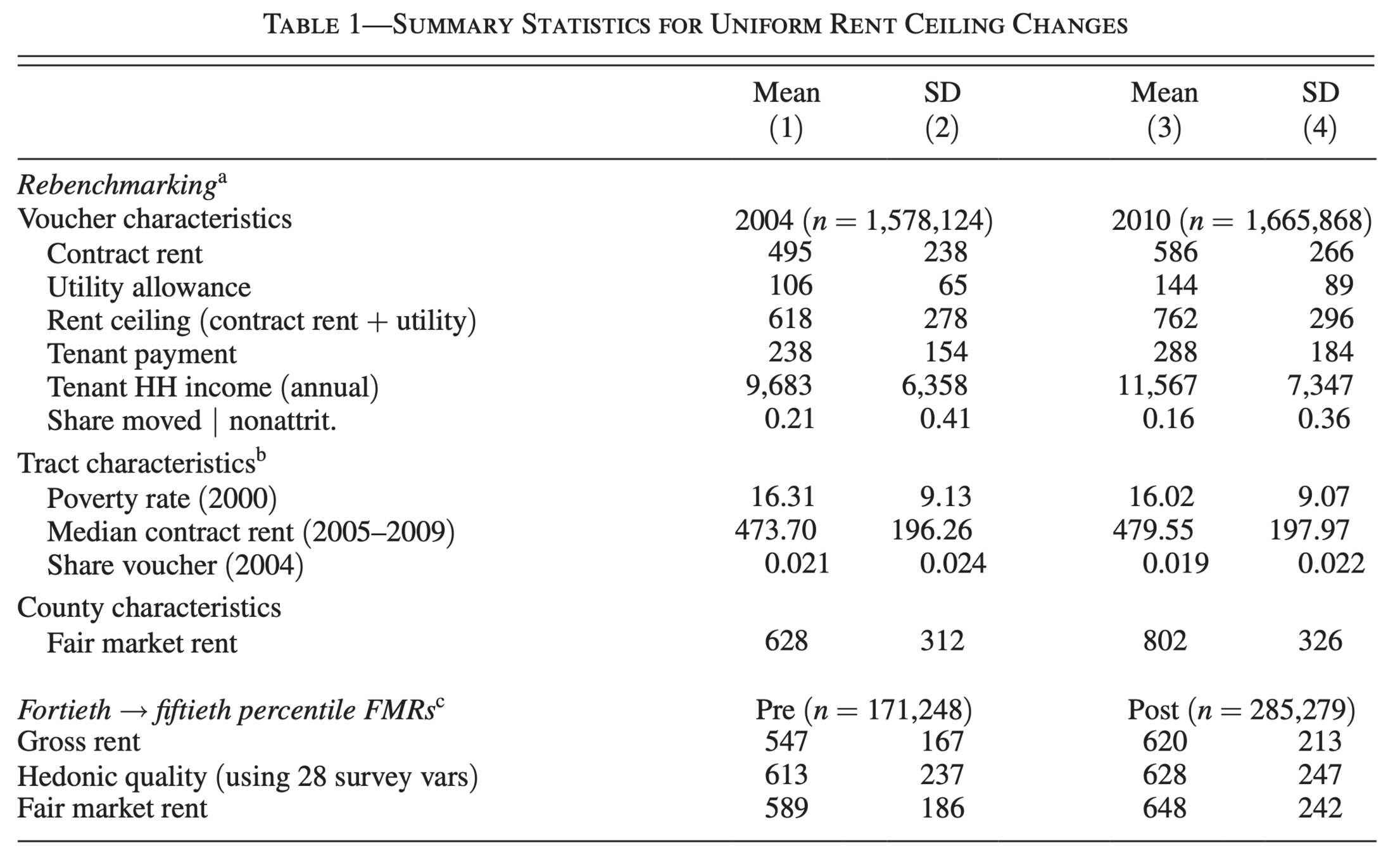
Consider the "rebenchmarking" of incorporating updated rents from the census as a "one-time, permanent change"
Estimation Equation
Interpretation
Note: The treatment variable is continuous, so I'm not going to write down the nonparametric form
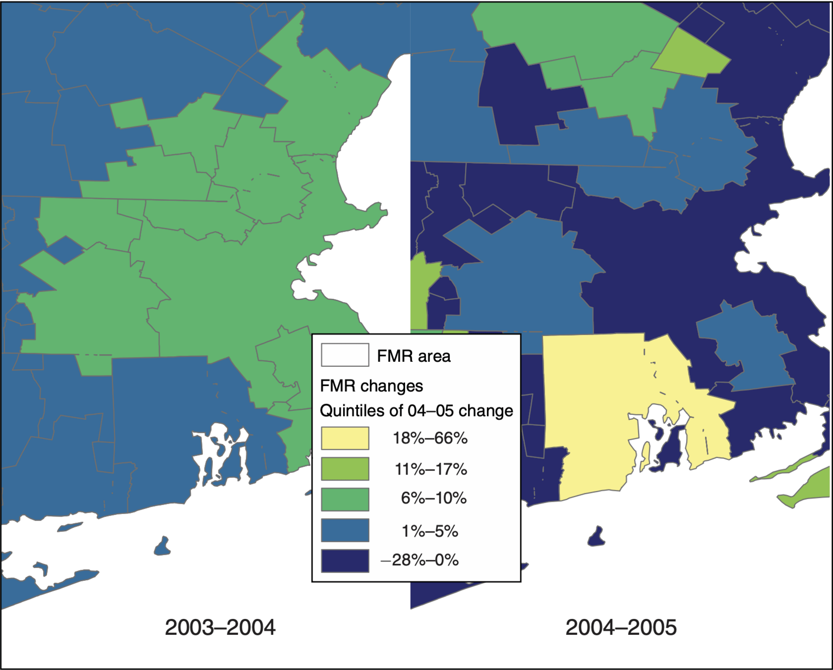
Conditioning on the Fair Market Rent in 2004 and the local housing authorities 2004 rent ceiling, we're capturing the residual term generated by the 2005 Fair Market Rent
What do you think about this source of variation?
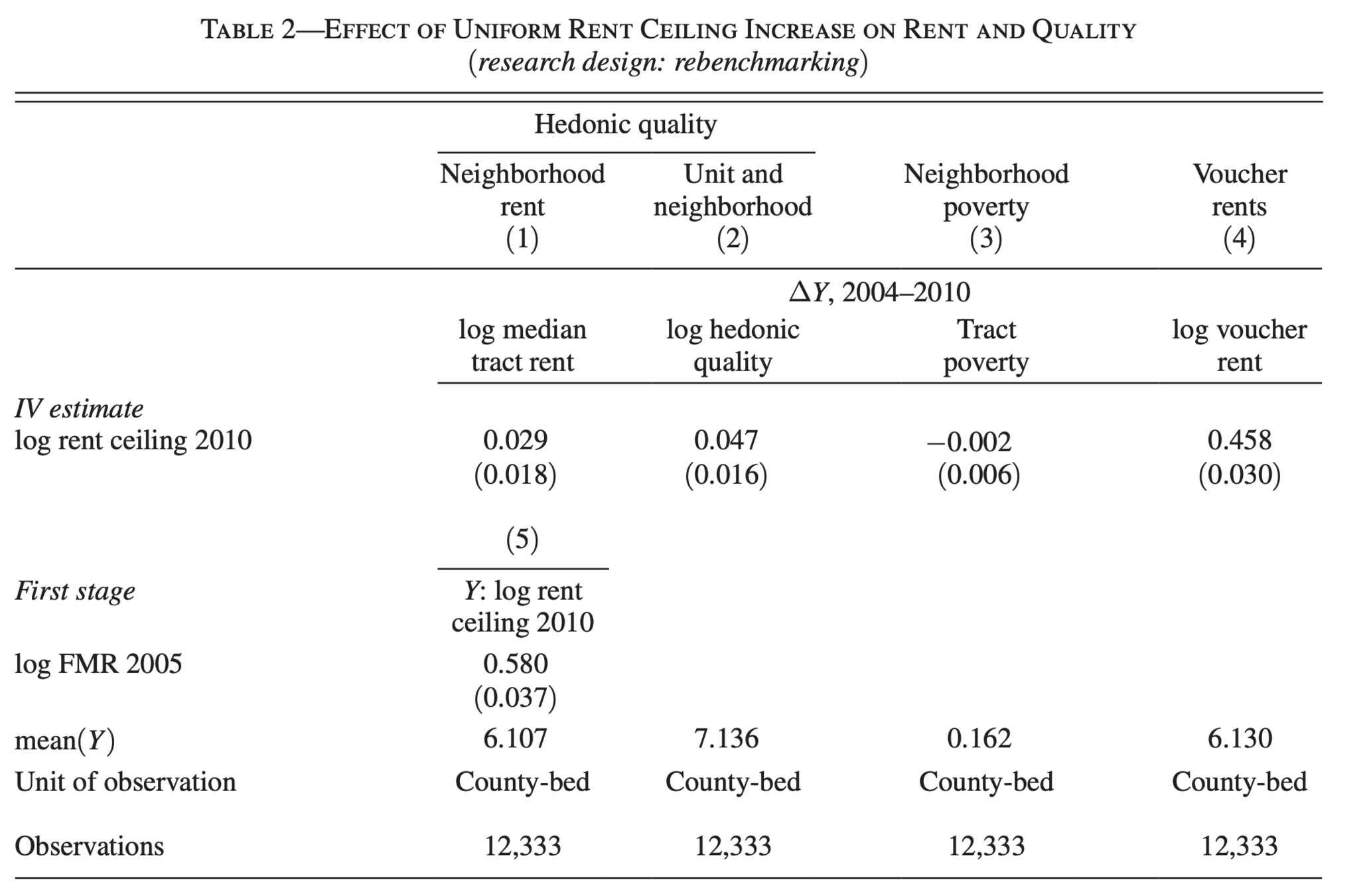
This coefficient drops to 0.15 when unit level fixed effects are included
Note, there are no tenant level controls
Uniform Rent Increases (Method 2)
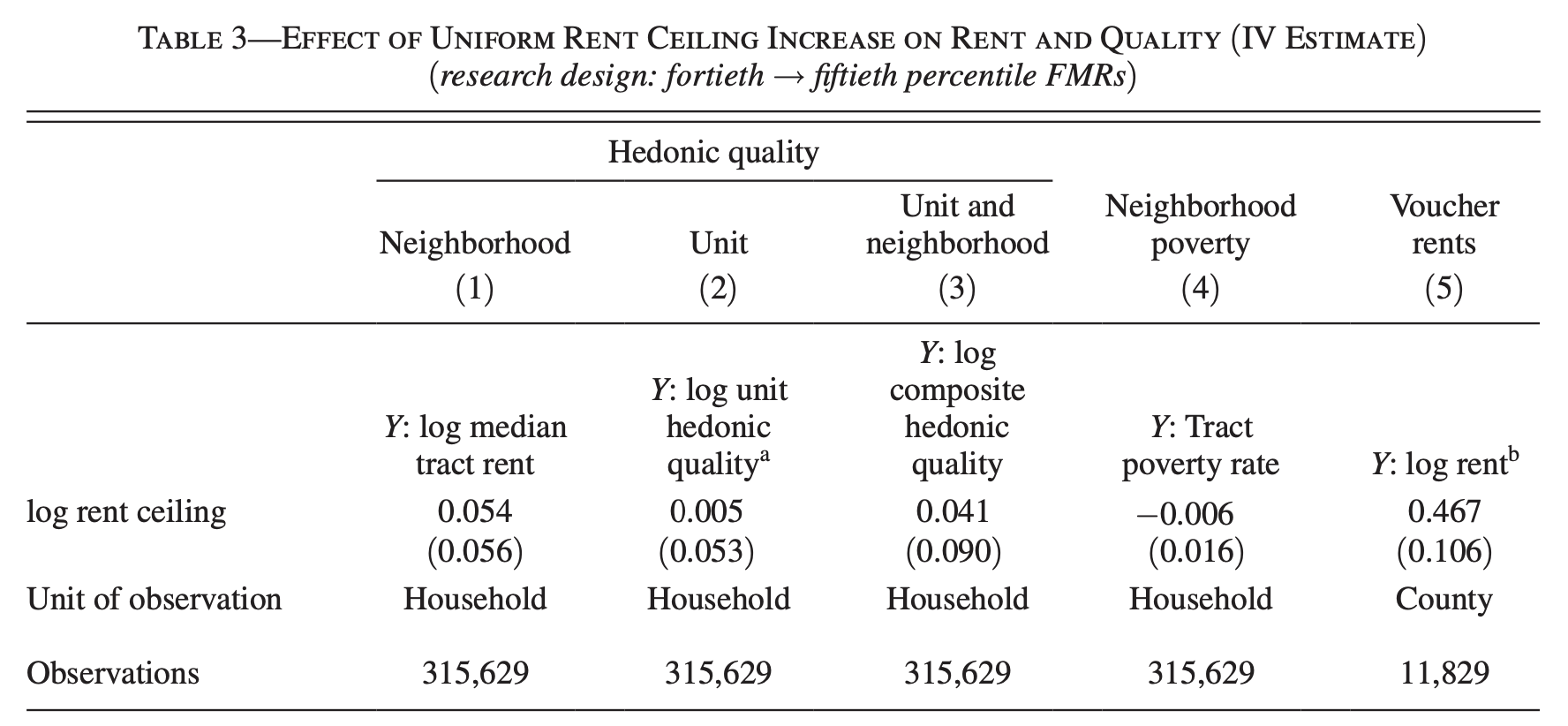
In 2001, HUD switched the FMR from the 40th percentile to the 50th percentile in 39 metro areas
Approach
Not exploiting non-parametric variation
What are the differences that these numbers capture?
(Surprising?!) Results
"We find that a policy of uniform increases in the ceiling raises the rents charged by voucher landlords to the government, with little impact on observed neighborhood quality"
Price
Quantity
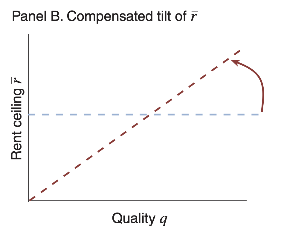
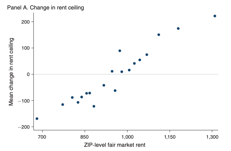
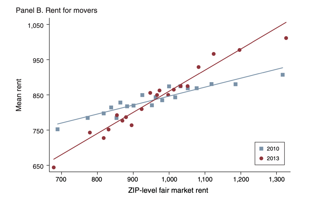
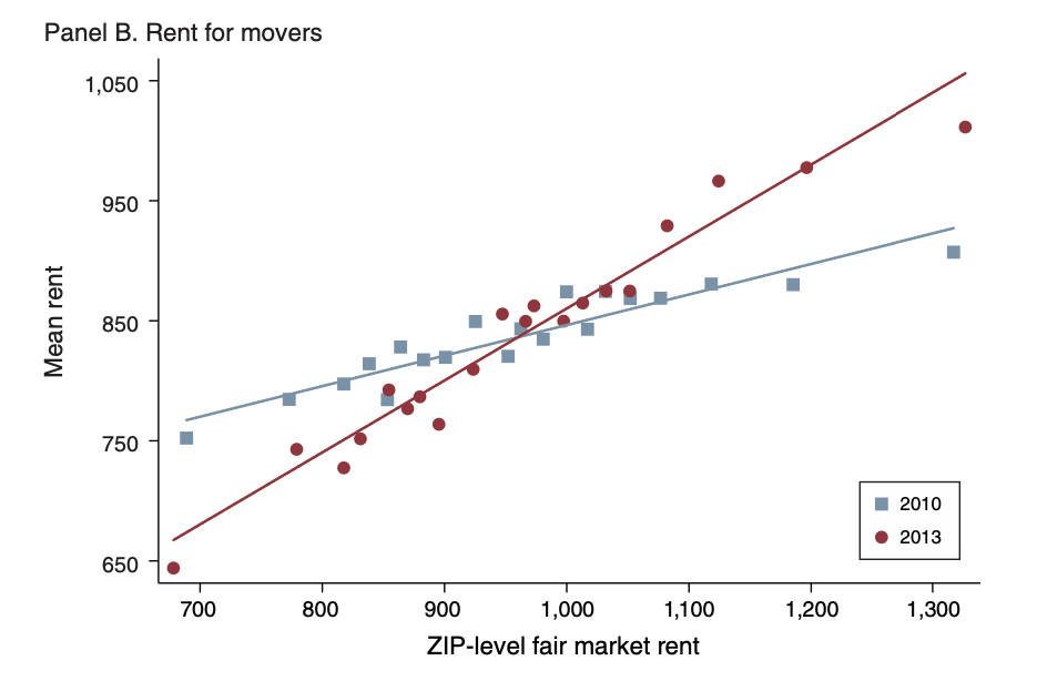
Tilting the Rent Ceiling
Target Rent Changes
Description
Result
Higher(lower) quality zip codes saw increases(decreases) in the Fair Market Rent
Rent
Neighborhood Quality
Notice the Writing: "a policy that establishes ZIP code-specific ceilings leads landlords to adjust rents"
?
Gold Standard
Randomize Rent Ceilings Across Zip Codes Within Housing Authorities
Approach
The shocks that we exploited before aren't quasi-random. FMR is correlated with area rent/quality
The shocks that we exploited before aren't quasi-random. FMR is correlated with area rent/quality
Method # 1
Nonparametrically, the residual term is 0 for 2011
This is continuous treatment difference-in-difference instrumental variables (Note how "far" we are from a simple randomized control trial)
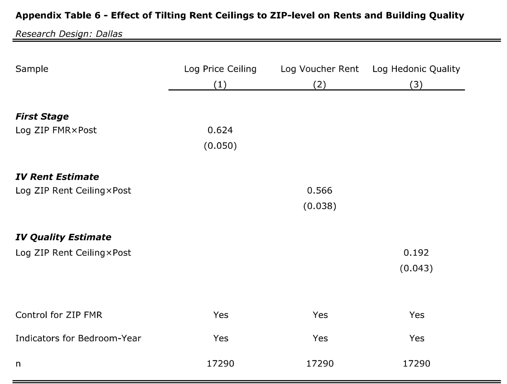
Method # 1
Estimand(s)
The impact of rent ceiling changes on rental price, housing quality and neighborhood
How should we define the treatment variable?
Relationships of Interest
Reflection Questions
Intuitively, the treatment variable should be an indicator for the fact that a tenant has a voucher from a Housing Authority which a tilted rent ceiling
And this should necessitate using tenant observations from outside of Dallas
Regression
Identification Assumption
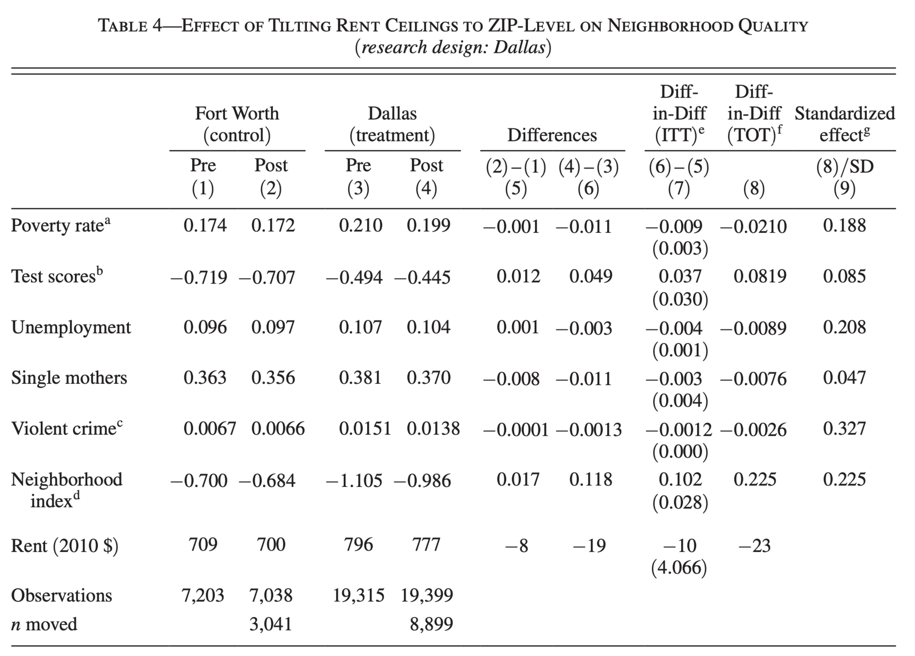
Are these time-invariant differences?
Compare these effects to the initial differences
Comparing policies
Thoughts
Intuitively, we have to and want to empirically compare policies
In practice, this is really hard without making strong assumptions
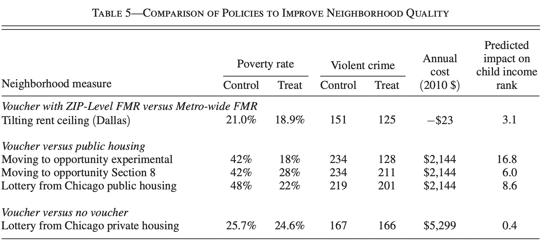
Ignores differences in Compliers
Key Assumption
The child lived in the new location from birth to age 20
(But we know from Chetty 2016 that this doesn't happen)
Additional Thoughts
What's the mechanism that explains why tenants move to higher quality neighborhoods when the FMR is slanted rather than increased uniformly?
How exactly does the supply side respond to increases?
Is there a displacement effect in the private market (i.e. musical chairs)
Is it that under a slanted FMR tenants cannot afford their current unit and therefore must relocate and in doing so strongly pursue higher quality neighborhoods?