Book 2. Credit Risk
FRM Part 2
CR 4. Capital Structure in Banks
Presented by: Sudhanshu
Module 1. Expected and Unexpected Loss
Module 2. Economic Capital for Credit Risk
Module 1. Expected and Unexpected Loss

Topic 1. Credit Risk Factors
Topic 2. Expected Loss (EL)
Topic 3. Unexpected Loss (UL)
Topic 4. Portfolio Expected & Unexpected Loss
Topic 1. Credit Risk Factors
-
Probability of default (PD / EDF): Measures the likelihood that a borrower defaults, but on its own it may not fully capture creditor risk, as some defaults can be temporary with little or no loss.
-
Exposure amount (EA / EAD): Represents the creditor’s exposure at default, stated as a dollar amount (e.g., outstanding loan balance) or as a percentage of the total loan or credit line.
-
Loss rate (LR / LGD): Measures the percentage loss incurred if default occurs, emphasizing that default severity matters as much as default likelihood.
-
LR = 1 − recovery rate (RR), and factors affecting LR also affect RR.
-
Topic 2. Expected Loss (EL)
-
Definition: The average or anticipated loss from a credit exposure over a time horizon.
-
Represents long-run statistical mean, not variability.
-
-
Formula & Components:
- EA (Exposure at Default): $ amount at risk
-
PD (Probability of Default): Likelihood of borrower default
-
LR (Loss Rate): Severity of loss if default occurs.
EL=EA×PD×LREL = EA \times PD \times LR
-
Expected vs unexpected loss: Expected loss (EL) reflects the average behavior of a risky asset, while actual asset values fluctuate around this average; the variability around EL is referred to as unexpected loss.
-
Sources of unexpected loss: Unexpected loss arises from default events or changes in credit quality (credit migration).
-
Modeling default risk: Default has a positive probability even for high-quality borrowers and can be estimated using historical data or structural models such as the Merton model, which treats equity as a call option on the firm’s assets.
-
Credit migration dynamics: Creditworthiness can deteriorate or improve over time; while migration may not trigger immediate default, it alters the future probability of default.
Topic 3. Unexpected Loss (UL)
- Definition: Variation in expected loss, modeled as deviation expected losses.
-
Captures risk of loss volatility due to uncertainty in defaults and recoveries.
-
Formula:
-
-
Variance of PD: Since we assume a two-state model, the variance of PD is simply the variance of a binomial random variable:
-
-
Analysis of UL formula:
-
The EA term explicitly recognizes that only the risky portion of the asset
is subject to default.
-
Each term is at most equal to one so the UL is a fraction of the exposure amount.
-
If the default and recovery are known with certainty, with their variations being 0, unexpected loss is equal to 0.
-
Practice Questions: Q1
Q1. XYZ Bank is trying to forecast the expected loss on a loan to a mid-size corporate borrower. It determines that there will be a 75% loss if the borrower does not perform the financial obligation. This risk measure is the:
A. probability of default.
B. loss rate.
C. unexpected loss.
D. exposure amount.
Practice Questions: Q1 Answer
Explanation: B is correct.
Current measures used to evaluate credit risk include the firm’s probability of default, which is the likelihood that a borrower will default, the loss rate, which represents the likely percentage loss if the borrower defaults, the exposure amount, and the expected loss, which, for a given time horizon, is calculated as the product of the EA, PD, and LR. The stated 75% loss if the borrower defaults is the loss rate.
Topic 4. Portfolio EL & UL
-
Portfolio EL: Sum of the expected losses of each asset:
- Additive across assets: Straightforward aggregation of expected average losses.
-
Portfolio UL Formula
- Incorporates correlation among assets.
- If
- Lower correlation → greater diversification → lower .
-
Risk Contribution: Risk contribution (RC), also known as unexpected loss contribution (ULC) is defined as:
- Shows marginal risk from each asset and sum of marginal risk of all assets = total portfolio risk
- Thus, isolates the incremental risk of adding asset i to the existing portfolio.∑IRCi=ULP \sum RC_i = UL_P
-
For a two-asset portfolio, the risk contributions of each asset are calculated as follows:
-
-
-
Together, the two risk contributions will equal the unexpected loss on the portfolio
-
-
-
Topic 4. Portfolio EL & UL
-
Diversifiable and Undiversifiable Risk
-
Risk of an isolated asset: An individual asset carries both diversifiable (firm-specific) risk and undiversifiable (market) risk.
-
Portfolio effect: In a well-diversified portfolio, firm-specific risk is largely eliminated as individual asset risks offset each other.
-
Residual risk: Undiversifiable risk remains as the asset’s residual contribution to overall portfolio risk and cannot be diversified away.∑IRCi=ULP \sum RC_i = UL_P
-
-
Effects of Correlation
-
Role of asset correlation: Higher correlation among bank assets increases concentration risk, as defaults can spill over across assets and amplify portfolio losses.
-
Need for reliable estimates: Accurate measurement of portfolio risk requires dependable estimates of default correlations.
-
Estimation challenges: Default correlations are difficult to assess in practice, especially between unrelated obligors, and the number of required pairwise calculations grows rapidly with portfolio size [n (n − 1)] / 2 covariances].
-
Example: 190 pairs for 20 assets and 4,950 pairs for 100 assets.
-
-
Topic 4. Portfolio EL & UL
-
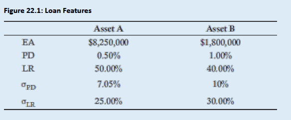
Example: Bigger Bank has two assets outstanding, with their features summarized in below Fig. Assuming a correlation of 0.3 between the assets, compute the expected loss and unexpected losses of the portfolio. Also calculate the risk contribution of each asset.
-
Solution
-
Step 1: Compute EL for both assets
-
-
Step 2: Compute UL for both assets
-
-
Step 3: Portfolio expected loss = $20,625 + $7,200 = $27,825
-
Step 4: Portfolio unexpected loss
-
-
-
Topic 4. Portfolio EL & UL
-
Example: Bigger Bank has two assets outstanding, with their features summarized in below Fig. Assuming a correlation of 0.3 between the assets, compute the expected loss and unexpected losses of the portfolio. Also calculate the risk contribution of each asset.
-
Solution
-
Step 5: Compute RC for both assets
-
-
-
Impact of correlation: If correlation between assets is reduced to 0.1, compute expected and unexpected losses of the portfolio:
-
As correlation does not impact each asset individually, the expected loss on the portfolio remains the same. However, the unexpected loss (variation) has decreased to $346,118.
Practice Questions: Q2
Q2. Which of the following statements about expected loss (EL) and unexpected loss (UL) is true?
A. Expected loss always exceeds unexpected loss.
B. Unexpected loss always exceeds expected loss.
C. EL and UL are parameterized by the exact same set of variables.
D. Expected loss is directly related to exposure.
Practice Questions: Q2 Answer
Explanation: D is correct.
EL increases with increases in the exposure amount. UL typically exceeds EL, but they are both equal to zero when probability of default is zero. UL has additional variance terms.
Practice Questions: Q3
Q3. If the recovery rate (RR) increases and the probability of default (PD) decreases, what will be the effect on expected loss (EL), all else equal?
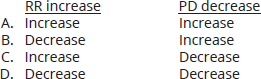
Practice Questions: Q3 Answer
Explanation: D is correct.
If recovery rates increase, the loss rate will decrease, which will decrease expected loss. If the probability of default decreases, the expected loss will also decrease.
Practice Questions: Q4
Q4. Big Bank has contractually agreed to a $20,000,000 credit facility with Upstart Corp., of which $18,000,000 is currently outstanding. Upstart has very little collateral, so Big Bank estimates a one year probability of default of 2%. The collateral is unique to its industry with limited resale opportunities, so Big Bank assigns an 80% loss rate. The expected loss (EL) for Big Bank is closest to:
A. $68,000.
B. $72,000.
C. $272,000.
D. $288,000.
Practice Questions: Q4 Answer
Explanation: D is correct.
Practice Questions: Q5
Q5. Bigger Bank has two assets outstanding. The features of the loans are summarized in the following table. Assuming a correlation of 0.2 between the assets, what is the value of the unexpected loss of the portfolio
A. Less than $300,000.
B. Between $300,000 and $400,000.
C. Between $400,000 and $500,000.
D. Greater than $500,000.
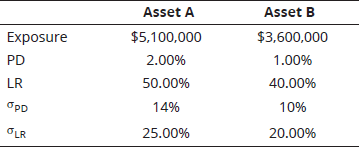
Practice Questions: Q5 Answer
Explanation: C is correct.
The following calculations describe the steps to compute the unexpected loss of a portfolio.
Compute UL for both assets:
Compute
Module 2. Economic Capital for Credit Risk
Topic 1. Economic Capital
Topic 2. Modeling Credit Risk
Topic 3. Challenges to Quantify Credit Risk
Topic 1. Economic Capital
- Need for capital buffers: Unexpected losses can far exceed expected losses, so banks must hold adequate capital reserves to absorb large shocks, avoid impairment, and continue operating.
-
Definition: The distance between the unexpected (negative) outcome and the expected outcome for a given confidence level (typically 99.97%).
-
The difference between the expected outcome and the confidence level can be estimated using the shape of the loss distribution
-
This difference can then be represented as a multiple of portfolio unexpected loss, which is often referred to as the capital multiplier (CM).
-
-
Formula:
Topic 2. Modeling Credit Risk
- Focus on tail risk: Economic capital for credit risk concentrates on the tail of the loss distribution, as credit losses are highly skewed with limited upside and rare but severe downside events.
-
Use of beta distribution: Credit losses are commonly modeled using a beta distribution since losses are bounded between 0% and 100%, and the distribution is flexible in shape based on its α and β parameters.
-
Interpretation of parameters: When α = β, the beta distribution is symmetric, with its mean and variance corresponding to expected loss (EL) and unexpected loss (UL), respectively.
-
Modeling extreme losses: The tail of the credit loss distribution is difficult to capture analytically and is often modeled by combining the beta distribution with Monte Carlo simulation.
Topic 3. Challenges to Quantify Credit Risk
-
Challenges in quantifying credit risk in bottom-up risk management approach:
- Illiquidity assumption: Bottom-up credit risk frameworks treat credits as illiquid assets, measuring losses at the portfolio level without fully capturing correlations among risk factors as seen in liquid markets.
-
Short modeling horizon: Practical credit risk models typically rely on a one-year horizon, despite credit quality evolving over multiple years, making longer-term modeling difficult to implement.
-
Risk silos: Credit risk is measured and managed separately from other risks (such as market and operational risk), leading to fragmented risk assessment across different bank functions.
Practice Questions: Q1
Q1. The type of capital used to buffer a bank from unexpected losses is known as:
A. economic capital.
B. regulatory capital.
C. unexpected capital.
D. risk-adjusted capital.
Practice Questions: Q1 Answer
Explanation: A is correct.
It is imperative that a bank hold capital reserves (i.e., economic capital) to buffer itself from unexpected losses so that it can absorb large losses and continue to operate.