Book 1. Foundations of Risk Management
FRM Part 1
FRM 6. The Arbitrage Pricing Theory and Multifactor Models of Risk and Return
Presented by: Sudhanshu
Module 1. Multifactor Model Assumptions and Inputs
Module 2. Applying Multifactor Models
Module 1. Multifactor Model Assumptions and Inputs

Topic 1. Capital Asset Pricing Model (CAPM)
Topic 2. Arbitrage Pricing Theory (APT)
Topic 3. Assumptions of APT
Topic 4. APT vs CAPM
Topic 5. Multifactor Model Inputs
Topic 1. Capital Asset Pricing Model (CAPM)
-
CAPM is a foundational model in finance that links an asset’s expected return to its market risk.
-
It assumes that all risk can be captured by a single factor: the market portfolio.
-
Investors are assumed to hold diversified portfolios that eliminate unsystematic (firm-specific) risk.
-
The formula for expected return:
-
where:
- Risk-free rate
- Asset's beta (senstivity to market)
- Expected market return
-
Limitations: CAPM ignores other sources of systematic risk beyond the market.
Topic 2. Arbitrage Pricing Theory (APT)
-
APT was proposed by Steven Ross in 1976 as a more flexible alternative to CAPM.
-
APT allows for multiple risk factors influencing asset returns, not just the market.
-
Factors can include macroeconomic variables such as:
-
Interest rate spreads
-
Inflation (expected vs actual)
-
Industrial production
-
Credit spreads
-
- The model assumes that in efficient markets, arbitrage opportunities are quickly exploited and eliminated.
- APT provides a linear relationship between expected return and multiple factor exposures.
-
The idea is to model systematic risk on a more granular level using a
series of risk factors.
Topic 2. Arbitrage Pricing Theory (APT)
-
The equation for APT is given as:
-
-
where
-
: actual return on stock i
-
: expected return on stock i
-
: beta (factor sensitivity) for factor 1
-
: first risk factor that could add return deviation from the expected return
-
: beta (factor sensitivity) for factor k
-
: last risk factor that could add return deviation from the expected return
-
: random error-term that accounts for company-specific (idiosyncratic) risk
-
Topic 3. Assumptions of APT
-
Market participants are seeking to maximize their profits.
-
Markets are frictionless (i.e., no barriers due to transaction costs, taxes, or lack of
access to short selling).
-
There are no arbitrage opportunities, and if any are uncovered, then they will be
very quickly exploited by profit-maximizing investors.
Topic 4. APT vs CAPM
-
CAPM is a single-factor model limited to market risk; APT is a multifactor model.
-
APT provides better real-world accuracy, especially when market risk is not the only concern.
-
CAPM offers elegance and simplicity but relies on stronger assumptions.
- APT requires estimation of multiple betas, but gives more detailed risk-return relationships.
- CAPM assumes all investors view the market similarly; APT allows individual perspectives on factor importance.
- CAPM is a special case of APT where only the market factor is used.
Practice Questions: Q1
Q1. Which of the following statements is correct regarding arbitrage pricing theory (APT)?
A. APT uses a pre-established series of variables to calculate expected returns.
B. APT provides more flexibility than traditional CAPM-based models.
C. APT relies on a stricter series of assumptions than the CAPM.
D. APT is constrained to a five-factor model.
Practice Questions: Q1 Answer
Explanation: B is correct.
Arbitrage pricing theory uses a completely customizable group of variables. It explicitly mixes the return of the market with a collection of macroeconomic variables. As such, it offers more granular flexibility than CAPM. It also uses much fewer restrictive assumptions than CAPM.
Topic 5. Multifactor Model Inputs
-
A multifactor model estimates asset returns based on exposure to several risk factors.
-
-
Inputs required:
- Factor values (e.g., change in GDP, inflation surprise)
- Factor sensitivities (betas) for each asset
-
Intercept term (alpha) – the asset’s expected return when all factors are zero
- Error term (epsilon) – captures unexpected firm-specific events
-
Example: A company might have strong sensitivity to GDP growth and consumer sentiment.
- If GDP surprises are negative and the company is highly sensitive to GDP, returns will drop.
- These models help isolate what portion of return is due to broad economic forces vs. company events.
Practice Questions: Q2
Q2. Which of the following statements regarding the inputs involved with a multifactor model is correct?
A. The factors included in a multifactor model are very rigid.
B. Factor betas describe how much the relationship is amplified between the stock under analysis and the respective factor.
C. Analysts must include only economic variables as the factors in a multifactor model.
D. Factor betas must be positive values.
Practice Questions: Q2 Answer
Explanation: B is correct.
Multifactor models include a series of factors and associated betas for each factor. The selection of factors is completely customizable with no constraints, and a beta factor can be positive or negative. In either instance, the beta factor will measure the relationship between the stock and the factor in question.
Module 2. Applying Multifactor Models
Topic 1. Calculating Expected Return – Single-Factor Model
Topic 2. Calculating Expected Return – Multifactor Model
Topic 3. Accounting for Correlation
Topic 4. Hedging Exposure to Multiple Factors
Topic 5. Challenges in Hedging Using Multifactor Models
Topic 6. The Fama-French Three-Factor Model
Topic 7. Applying the Fama-French Model – Example
Topic 1. Calculating Expected Return – Single-Factor Model
-
In a single-factor model, expected return depends on one factor.
-
Example:
-
-
HealthCare Inc (HCI) has an expected return of 10%.
-
Beta to GDP = 2.0
-
Expected GDP = 3.2%, actual = 2.6% → Surprise = -0.6%
-
Return impact = 2.0 × (−0.6%) = −1.2%
-
Adjusted expected return = 10% − 1.2% = 8.8%
-
- Difference between predicted and actual return indicates missing risk factors or firm-specific events.
- This model assumes only one factor affects the return, which is often insufficient.
Topic 2. Calculating Expected Returns – Multifactor Model
-
Now we add another factor, like consumer sentiment (CS).
-
-
-
Beta to consumer sentiment (CS) = 1.5
-
Expected CS = 1.0%, Actual = 0.75% → Surprise = −0.25%
-
CS Impact = 1.5 × −0.25% = −0.375%
-
Updated expected return: 8.8% − 0.375% = 8.43%
-
This model captures more systematic effects and results in more accurate predictions.
-
Adding further relevant factors (e.g., inflation or energy prices) can improve accuracy even more.
Practice Questions: Q3
Q3. What value is derived from adding more factors through a multifactor approach?
A. All company-specific risk can be mitigated.
B. The same variables can be added for every stock, which makes the process easy to implement.
C. Calculations can be derived over multiple time periods because the factor betas remain static.
D. A richer systematic relationship can be captured.
Practice Questions: Q3 Answer
Explanation: D is correct.
Adding multiple risk factors does not eliminate company-specific risk, which is also known as nondiversifiable risk. Each stock will use its own variables, so an analyst will need to source variables for each stock under review and periodically check (and maybe change) the factors deployed because the factors and the factor betas are dynamic over time. Adding multiple risk factors does enhance the discovery of systematic risk influence.
Topic 3. Accounting for Correlation
-
APT assumes portfolios are well-diversified to eliminate firm-specific risk.
-
Diversification is most effective when correlation between assets is low.
-
Assets from different industries or asset classes tend to have lower correlation.
-
Correlation matters because it influences how much risk remains after diversification.
-
A multifactor model benefits when different assets respond differently to each factor.
-
The more uncorrelated the asset returns are, the more useful a multifactor approach becomes.
Practice Questions: Q4
Q4. Which of the following statements about correlation and diversification is correct with respect to multifactor models?
A. Well-diversified portfolios hold constituent assets with high correlations.
B. The use of well-diversified portfolios removes the need for multifactor models.
C. The use of multiple assets with lower correlations makes the use of multifactor models more beneficial for analysts to consider.
D. Well-diversified portfolios typically include assets from the same asset class.
Practice Questions: Q4 Answer
Explanation: C is correct.
APT requires a well-diversified portfolio, which means that assets with lower correlations coming from different asset categories need to be included. This requirement will broaden the pool of influential factors and make a multifactor model a more attractive option. Using uncorrelated assets can lessen but not eliminate company-specific risk.
Topic 4. Hedging Exposure to Multiple Factors
- Multifactor models allow custom hedging of specific risk exposures.
- Investor can neutralize exposure to certain factors without selling the whole portfolio.
-
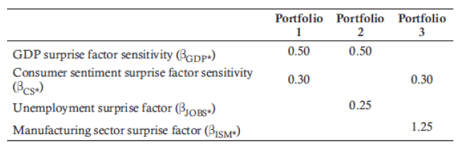
Consider below example with three well-diversified portfolios
-
An investor could take a long position in Portfolio 1 and a short position in Portfolio 2.
-
Doing so would result in a zero beta for GDP surprise, but it would retain a 0.30 beta for consumer sentiment surprise and add a −0.25 beta (because the position is held short) to unemployment surprise.
-
It is possible to find a financial asset that only has an equal factor exposure to the single variable of GDP surprise.
-
Practice Questions: Q5
Q5. Which of the following statements relative to the use of multifactor models and hedging is incorrect?
A. Multifactor models enable investors to hedge specific factor exposures.
B. There are still no arbitrage opportunities, even when factoring in the granular exposures captured by multifactor models.
C. Multifactor models potentially enable investors to eliminate all calculated factor exposures.
D. The hedging process will most likely contain an element of model risk.
Practice Questions: Q5 Answer
Explanation: B is correct.
The use of multifactor models enables investors to focus on granular risk exposures. Investors can hedge a single exposure and retain the others. They can also potentially hedge all calculated risk exposures. This process could produce arbitrage opportunities given the right circumstances. Because this hedging process is based on the calculated model, there will always be an element of model risk.
Topic 5. Challenges in Hedging Using Multifactor Models
- Model Risk: Incorrect factor selection or inaccurate beta estimation.
-
Rebalancing:
- Too frequent = High transaction costs.
- Too infrequent = Exposure to unhedged risks.
- Assumption of stationarity (i.e., stable relationships over time) may not hold.
Topic 7. The Fama-French Three-Factor Model
- Developed by Eugene Fama and Kenneth French as an extension to CAPM.
-
Adds two factors to better explain stock returns:
- SMB (Small Minus Big) – Captures size effect; small-cap stocks often outperform.
- HML (High Minus Low) – Captures value effect; high book-to-market stocks often outperform.
-
Model:
-
- Market risk remains the core component (like CAPM), but size and value effects improve accuracy.
- Any return that is different from this calculation is considered to be alpha (α).
- Both SMB and HML are constructed as long-short portfolios, making the model self-neutralizing.
- These effects are observed across long-term historical data.
Practice Questions: Q6
Q6. Which factors are explicitly considered in the Fama-French three-factor model?
A. A size factor.
B. A momentum factor.
C. A currency exposure factor.
D. An operational robustness factor.
Practice Questions: Q6 Answer
Explanation: A is correct.
The Fama-French three-factor model explicitly adjusts for size (SMB) and valuation (HML). Carhart added a momentum factor one year after Fama and French’s original work. Fama and French also added an operating profit measure and an investment conservatism factor in a very recent extension of their own work.
Topic 8. Applying the Fama-French Model – Example
-
Suppose a stock has the following factor sensitivities:
- Market beta = 0.85
- SMB beta = 1.65
- HML beta = −0.25
- Market premium = 8.5%, SMB = 2.5%, HML = 1.75%, Risk-free rate = 2.75%
-
Plug into the model:
- E(R)=2.75+(0.85×8.5)+(1.65×2.5)−(0.25×1.75)
- E(R)=2.75+7.225+4.125−0.4375=13.66%E(R) = 2.75 + 7.225 + 4.125 − 0.4375 = \textbf{13.66\%}E(R)=2.75+7.225+4.125−0.4375=13.66%
- Any difference between actual return and 13.66% is alpha, which could signal mispricing or missing factors.