Book 5. Risk and Investment Management

FRM Part 2

IM 3. Alpha (and the Low-Risk Anomaly)

Presented by: Sudhanshu

Module 1. Low-Risk Anomaly, Alpha and the Fundamental Law of Active Investment

Module 2. Factor Regression and Portfolio Sensitivity

Module 3. Time-Varying Factors, Volatility and Beta Anomalies, and Anomaly Explanations

Module 1. Low-Risk Anomaly, Alpha and the Fundamental Law of Active Investment

Topic 1. Low-Risk Anomaly

Topic 2. Alpha and Tracking Error,

Topic 3. Information Ratio and Sharpe Ratio

Topic 4. Benchmark Selection for Alpha

Topic 5. Fundamental Law of Active Management

Topic 1. Low-Risk Anomaly

Traditional Finance (CAPM): States that there should be a positive relationship between risk (measured by beta) and return. Higher risk should lead to higher returns.
Low-Risk Anomaly: In practice, the opposite has been observed. Firms with lower betas and lower volatility tend to have higher returns over time.
Evidence of the Low-Risk Anomaly: Over a 5-year period from 2011–2016, the cumulative return for a low volatility fund (iShares Edge MSCI Minimum Volatility USA ETF) was 68.75% relative to the cumulative return of 65.27% for the S&P 500 Index ETF.

Practice Questions: Q1

Q1. Which of the following statements is correct concerning the relationship between the low-risk anomaly and the capital asset pricing model (CAPM)?

A. The low-risk anomaly provides support for the CAPM.

B. The notion that the low-risk anomaly violates the CAPM has not been proven empirically.

C. The low-risk anomaly violates the CAPM and suggests that low-beta stocks will outperform highbeta stocks.

D. Both CAPM and the low-risk anomaly point to a positive relationship between risk and reward.

Practice Questions: Q1 Answer

Explanation: C is correct.

The low-risk anomaly violates the CAPM and suggests that low beta stocks will
outperform high-beta stocks. This has been empirically proven with several
studies. The CAPM points to a positive relationship between risk and reward, but the low-risk anomaly suggests an inverse relationship.

Topic 2. Alpha and Tracking Error

Defining Alpha
- Alpha ( $α$ ): The return earned in excess of a benchmark. It is a measure of average performance relative to a benchmark and
- Alpha is also called as active return and benchmark is called as passive return.
- Excess Return ( ): The difference between the return of an asset ( $R_{t}$ ) and the return of its benchmark
- Calculation: Alpha is the average of the excess returns over a period of $T$ observations.
- Investor Skill: While often interpreted as a measure of skill, it is fundamentally a statement of performance against a specific benchmark.
Tracking Error
- Tracking Error : The standard deviation of excess returns.
- Measures the dispersion of an investor's returns relative to their benchmark.
- A larger tracking error indicates more freedom in decision-making.

R_t^{ex}

R_t^{ex}=R_t-R_t^B

\alpha=\frac{1}{T}\sum_{t=1}^T R_t^{ex}

(\bar{\sigma})

\text{tracking error} =\bar{\sigma}= \text{standard deviation} \left(R_t^{\mathrm{ex}}\right)

Information Ratio (IR):
- A measure of risk-adjusted returns for active managers.
- It standardizes alpha using the tracking error.
- Used to rank active investment choices.
Sharpe Ratio:
- A measure of risk-adjusted return when the risk-free rate ( $R_{F}$ ) is used as the benchmark.
- Calculation:
  - is the portfolio return.
  - $R_{F}$ is the risk-free rate.
  - $σ_{p}$ is the standard deviation of the portfolio.

IR=\frac{\alpha}{\bar{\sigma}}

\text{Sharpe Ratio= }\frac{R_p-R_F}{\sigma_P}

R_p

Topic 3. Information Ratio and Sharpe Ratio

Topic 4. Benchmark Selection for Alpha

The Importance of Benchmark Choice
- Impact on Alpha: The choice of benchmark significantly affects the calculated alpha.
- The Beta Problem: A simple benchmark like the S&P 500 Index assumes a beta of 1.0. If an investment's true beta is different (e.g., 0.73), using the wrong benchmark will understate the true alpha and Information Ratio.
- Example: An investment with a beta of 0.73 and a true alpha of 3.44% would be incorrectly calculated as having an alpha of 1.50% if a simple S&P 500 benchmark (assuming a beta of 1.0) is used.
Characteristics of an Effective Benchmark
- Well-Defined: Should be hosted by an independent index provider, making it verifiable and free of ambiguity (e.g., S&P 500 Index).
- Tradeable: Must be a basket of tradeable securities that an investor could invest in as an alternative.
- Replicable: Closely related to tradability, an investor must be able to replicate the benchmark.
- Risk-Adjusted: The benchmark's risk level must be appropriate for the investment in question. Failing to adjust for risk can lead to an understated alpha.

Practice Questions: Q2

Q2. Which of the following statements is not a characteristic of an appropriate benchmark? An appropriate benchmark should be:

A. tradeable.

B. replicable.

C. well-defined.

D. equally applied to all risky assets irrespective of their risk exposure.

Practice Questions: Q2 Answer

Explanation: D is correct.

An appropriate benchmark should be well-defined, replicable, tradeable, and risk- adjusted. If the benchmark is not on the same risk scale as the assets under review, then there is an unfair comparison.

Topic 5. Fundamental Law of Active Management

Grinold's Fundamental Law of Active Management
- Purpose: A mechanism for systematically evaluating investment strategies by formalizing the relationship between a manager's active bets and potential alpha.
- The Law:
  - IR: Information Ratio.
  - IC (Information Coefficient): The correlation between a manager's predicted value and the actual value. It is an explicit evaluation of forecasting skill. A higher IC means higher-quality predictions.
  - BR (Breadth): The number of independent investment bets deployed.
- The Tradeoff: The law highlights a central tradeoff: investors must either "play smart" (high IC) or "play often" (high BR) to achieve a desired Information Ratio.
Key Assumption: The law ignores downside risk and assumes that all forecasts are independent of one another
Limitation: In practice, as assets under management increase, the IC tends to decline. This can lead to decreased performance, which is why some funds close to new investors.

IR \approx IC \times \sqrt{BR}

Practice Questions: Q3

Q3. Grinold's fundamental law of active management suggests that:

A. investors should focus on increasing only their predictive ability relative to stock price movements.

B. sector allocation is the most important factor in active management.

C. a small number of investment bets decreases the chances of making a mistake and, therefore, increases the expected investment performance.

D. to maximize the information ratio, active investors need to either have high-quality predictions or place a large number of investment bets in a given year.

Practice Questions: Q3 Answer

Explanation: D is correct.

Grinold’s fundamental law of active management focuses on the tradeoff of high quality predictions relative to placing a large number of investment bets. Investors can focus on either action to maximize their information ratio, which is a measure of risk-adjusted performance. While sector allocation is a very important component of the asset allocation decision, Grinold focused only on the quality of predictions and the number of investment bets made.

Module 2. Factor Regression and Portfolio Sensitivity

Topic 1. Factor Regression to Construct a Benchmark: CAPM

Topic 2. Factor Regression to Construct a Benchmark: Fama-French Three Factor Model

Topic 3. Momentum Factor and Challenge of Using the Fama-French Model

Topic 1. Factor Regression to Construct a Benchmark: CAPM

Factor regression can be applied to construct a benchmark with multiple factors, extending the CAPM
CAPM-based Regression:
- This regression implies a benchmark that is a blend of the risk-free rate and the market return.
Using regression, alpha ( $α$ ) is approximated by regressing the excess return of the asset $(R_{i, t} - R_{F})$ against the excess return of the market $(R_{M} - R_{F})$ :

$R_{i, t} - R_{F} = α + β (R_{M} - R_{F}) + ϵ_{i, t}$
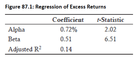
$This analysis was conducted for Berkshire Hathaway (Jan 1990-May 2012) relative to S&P 500, and the regression yield an$ α=0.72% and $β = 0.51. Thus,$ the regression implies the CAPM equation as:
- $R_{B}$ $=0.49 R_{F} +0. 51 R_{M}$ => α = $R_{i}$ $-[0.49 R_{F}$ +0.51E( $R_{M}$ $)]$
$It can be interpreted that a customized benchmark of 49% in the risk-free asset and 51% in the market$ would produce an expected alpha of 0.72% per month.

R_B = E\left(R_i\right)=R_F+\beta\left[E\left(R_M\right)-R_F\right] \implies R_B= (1-\beta) \mathrm{R}_{\mathrm{F}}+ \beta \mathrm{E}\left(\mathrm{R}_{\mathrm{M}}\right)

Fama-French Three-Factor Model: The CAPM-based regression is extended to include two additional factors for size and value/growth effects:
- Size effect (SMB): "Small minus big" => Return on small stocks minus the return on big stocks.
  - This is a long-short factor: $1 long in small caps and $1 short in large caps.
  - The SMB beta is positive for co-movement with small stocks, negative for large stocks, and zero for medium companies with no co-movement with either small or large stocks.
- Value/Growth effect (HML): "High minus low" => Represents the value premium (high minus low book-to-market stocks).
  - This is a long-short factor: $1 long in value and $1 short in growth stocks.
  - The HML beta will be positive if the assets have a value focus, and it will be negative if the assets have a growth focus.
The Fama-French three-factor model is constructed as follows:

Topic 2. Factor Regression to Construct a Benchmark: Fama-French Three Factor Model

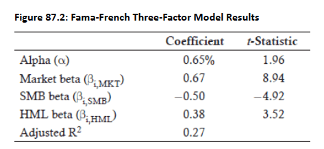
R_i-R_F=\alpha+\beta_{i, M K T} \times\left(R_M-R_F\right)+\beta_{i, S M B} \times(S M B)+\beta_{i, H M L} \times(H M L)

Fama-French model was applied to Berkshire Hathaway (Jan 1990–May 2012), results in Fig 87.2:
- Alpha declined slightly but remains very high, while market beta increased from 0.51 to 0.67. The negative SMB beta suggests a large company bias, and the positive HML beta indicates a value investing focus.
- The adjusted R² rose from 0.14 to 0.27, indicating that SMB and HML factors add explanatory value to the model. These results enable construction of a custom benchmark for Berkshire Hathaway implied by the Fama-French three-factor model.
All the factor weights in this formula sum to 1.0, but adding the SMB and HML factors add explanatory ability to the regression equation.

Topic 2. Factor Regression to Construct a Benchmark: Fama-French Three Factor Model

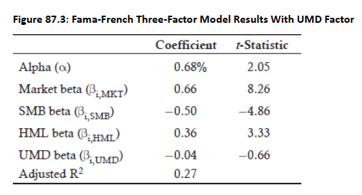
\begin{aligned} \mathrm{R}_{\mathrm{B}}= & 0.33(\mathrm{~T}-\text { bills })+0.67 \times(\text { market portfolio })-0.5(\text { small caps }) \\ & +0.5(\text { large caps })+0.38(\text { value stocks })-0.38(\text { growth stocks })\end{aligned}

Momentum Factor: A fourth factor, UMD, can be added to the Fama-French model to account for the momentum effect, where upward trending stocks continue rising and downward trending stocks continue falling.
- UMD (Up Minus Down) represents upward trending stocks minus downward trending stocks.
- A positive UMD beta indicates focus on upward trending stocks, a negative UMD beta indicates focus on downward trending stocks, and a beta of zero suggests no relationship.
- Analysis shows that Berkshire Hathaway does not have exposure to momentum investing.
A core challenge with the Fama-French model is index replication, as the SMB and HML indices created by Fama and French are conceptual and not directly tradeable. Including only tradeable factors is critical because the factors chosen greatly influence the calculated alpha.

Topic 3. Momentum Factor and Challenge of Using the Fama-French Model

Practice Questions: Q1

Q1. Why would an investor include multiple factors in a regression study?

I. To attempt to improve the adjusted measure.

II. To reduce the t-stat value on the respective regression coefficients.

A. I only.

B. II only.

C. Both I and II.

D. Neither I nor II.

R^2

Practice Questions: Q1 Answer

Explanation: A is correct.

An investor should consider adding multiple factors to the regression analysis to potentially improve the adjusted measurement, potentially increase the tests of statistical significance, and to search for a benchmark that is more representative of a portfolio’s investment style.

R^2

Module 3. Time-Varying Factors, Volatility and Beta Anomalies, and Anomaly Explanations

Topic 1. Measurement of Time-Varying Exposure Using Style Analysis

Topic 2. Issues With Alpha Measurement for Nonlinear Strategies

Topic 3. Volatility and Beta Anomalies

Topic 4. Potential Explanations for Risk Anomaly

Topic 1. Measurement of Time-Varying Exposure Using Style Analysis

Style analysis is a form of factor benchmarking where the factor exposures evolve over time.
Unlike Fama and French’s untradeable SMB and HML indices, style analysis uses tradeable assets.
For example, consider three funds: (1) SPDR S&P 500 ETF (SPY), (2) SPDR S&P 500 Value ETF (SPYV), and (3) SPDR S&P 500 Growth ETF (SPYG).
Style analysis also adjusts for the fact that factor loadings (betas) change over time.
A possible multifactor regression could be estimated for next period’s expected asset return as follows:
This formula has an imposed restriction that all factor loadings (i.e., factor weights) must sum to one:
The time-varying portion of this equation comes into play with the respective factor loadings. This process uses estimates that incorporate information up to time t.
Every new month (t + 1) requires a new regression to adjust the factor loadings. This means that the beta factors will change over time to reflect changes in the real world.

1=\beta_{\mathrm{SPY}, \mathrm{t}}+\beta_{\mathrm{SPYV}, \mathrm{t}}+\beta_{\mathrm{SPYG}, \mathrm{t}}

\mathrm{R}_{\mathrm{t}+1}=\alpha_{\mathrm{t}}+\beta_{\mathrm{SPY}, \mathrm{t}} \mathrm{SPY}_{\mathrm{t}+1}+\beta_{\mathrm{SPYV}, \mathrm{t}} \mathrm{SPYV}_{\mathrm{t}+1}+\beta_{\mathrm{SPYG}, \mathrm{t}} \mathrm{SPYG}_{\mathrm{t}+1}+\varepsilon_{\mathrm{t}+1}

R_{t+1}

Alpha is computed using linear regression, which can incorrectly suggest alpha exists for nonlinear strategies like uncovered long put options with L-shaped payoff profiles.
False positive alpha occurs when payoffs involve quadratic terms ( ) or option-like terms such as max( ), creating significant problems for hedge fund strategies like merger arbitrage, pairs trading, and convertible bond arbitrage with nonlinear payoffs.
Nonlinear strategies yield false positive alpha because return distributions are non-normal and often exhibit negative skewness, increasing left-tail loss potential and thickening the middle distribution.
Skewness is not factored into alpha calculations, creating measurement issues for nonlinear payoff strategies.

Topic 2. Issues With Alpha Measurement for Nonlinear Strategies

R_{t}^2

R_t,0

Topic 3. Volatility and Beta Anomalies

Haugen and Heins (1975) found using 1926-1971 data that stock portfolios with lower monthly return variance experienced greater average returns than riskier counterparts over the long run.
Ang et al. (2006) found a volatility anomaly using September 1963-December 2011 data organized into quintiles: as standard deviation increased, average returns decreased from 10%+ for the lowest three quintiles to 6.8% (quintile 4) and 0.1% (highest volatility), while Sharpe ratios declined from 0.8 to 0.0.
Initial 1970s CAPM testing found positive relationships between beta and expected returns, but Ang et al. (2006) later found high-beta stocks have lower risk-adjusted returns with Sharpe ratios falling from 0.9 (lowest betas) to 0.4 (highest betas).
The beta anomaly indicates higher-beta stocks have lower Sharpe ratios due to higher volatility (standard deviation in denominator) paired with higher betas, not necessarily lower absolute returns.
CAPM predicts contemporaneous (not predictive) relationships between beta and returns during the same measurement period; the challenge is that historical betas poorly predict future betas, limiting their usefulness for expected return predictions.
Buss and Vilkov (2012) found some improvement using implied volatility from option pricing models to estimate future betas over historical betas, though the beta anomaly remains primarily a challenge in reliably predicting future betas.

Topic 4. Potential Explanations for Risk Anomaly

The risk anomaly's explanation likely involves a combination of data mining, investor leverage constraints, institutional manager constraints, and preference theory, though no single comprehensive explanation exists.
Data mining is not well-supported as the sole explanation; the risk anomaly appears during recessions and expansions, across U.S. and international stocks, Treasury and corporate bonds, and in options and commodity markets.
Leverage-constrained investors (particularly retail investors unable to borrow) invest in high-beta stocks for built-in leverage, bidding up prices until assets become overvalued with decreased risk-adjusted returns, while low-beta stocks have lower prices and higher risk-adjusted returns.
Institutional manager constraints include restrictions against short selling and tracking error limits that prevent capturing perceived alpha by going long undervalued portfolios and short overvalued ones, with changing benchmarks or tolerance bands being difficult processes requiring investment committee approval.
Investor preference for high-volatility, high-beta stocks (often driven by bullish expectations) bids up prices and lowers future returns, while creating attractive entry points for long-term investors seeking lower volatility investments.
Heterogeneous investor preferences and investment constraints explain part of the risk anomaly; when disagreement is low with long-only constraints, CAPM holds best, but high disagreement leads to overpriced investments, decreased future returns, and potential inverse relationships between beta and returns.

Practice Questions: Q1

Q1. Which of the following characteristics is a potential explanation for the risk anomaly?

A. Investor preferences.

B. The presence of highly leveraged retail investors.

C. Lack of short selling constraints for institutional investors.

D. Lack of tracking error constraints for institutional investors.

Practice Questions: Q1 Answer

Explanation: A is correct.

Potential explanations for the risk anomaly include: the preferences of investors, leverage constraints on retail investors that drive them to buy pre-leveraged investments in the form of high-beta stocks, and institutional investor constraints like prohibitions against short selling and tracking error tolerance bands.