Copy of MR 15. Art of Term Structure Models- Volatility and Distribution

Book 1. Market Risk

FRM Part 2

MR 15. Art of Term Structure Models- Volatility and Distribution

Presented by: Sudhanshu

Module 1. Time-Dependent Volatility Models

Module 2. Cox-Ingersoll-Ross (CIR) and Lognormal Models

Module 1. Time-Dependent Volatility Models

Topic 1. Short-term Rate process

Topic 2. Short-term Rate change and Behaviour of Standard Deviation of Rate Change

Topic 3. Model 3 Effectiveness

Topic 1. Short-term Rate Process

The generic continuously compounded instantaneous rate,

$r_{t}$ , changes over time according to the relationship: $d r = λ (t) d t + σ (t) d w$ .
This model extends Model 1 (with no drift) by including time-dependent drift and volatility:
- $d r = σ d w$ becomes $d r = λ (t) d t + σ (t) d w$ .
It also extends the Ho-Lee model by incorporating non-constant volatility
- $d r = λ (t) d t + σ d w$ now includes $σ (t)$ .
In these models, $d w$ is normally distributed with a mean of 0 and a standard deviation of

\sqrt{dt}

Topic 2. Short-term Rate Change and Behavior of Standard Deviation of Rate Change

The relationships between volatility in each period can take on a nearly limitless number of combinations.
For example, the volatility of the short-term rate in one year, σ(1), could be 220 basis points and the volatility of the short-term rate in two years, σ(2), could be 260 basis points.
To make the analysis tractable, a specific parameterization of time-dependent volatility is assigned, such as Model 3.
Model 3:
- $σ$ represents volatility at $t = 0$ , which exponentially decreases to 0 for $α > 0$ .
Example Calculation (Model 3):
- Given $r_{0} = 5%$ , $λ = 0.24%$ , $σ = 1.50%$ , $α = 0.3$ , and $d w = 0.2$ (for one month, $d t = 1/12$ ).
- The new short-term rate is:
- This value is slightly less than with constant volatility (5.32%), due to the exponential decay in volatility.

d r=\lambda(t) d t+\sigma e^{-\alpha t} d w

d r=0.24 \% \times(1 / 12)+1.5 \% \times e^{-0.3(1 / 12)} \times 0.2 =0.02 \%+0.29 \%=0.31 \%

5\%+0.31\%=5.31\%

Topic 3. Model 3 Effectiveness

Time-dependent volatility models offer increased flexibility for modeling future short-term rates.
They are especially useful for pricing multi-period derivatives like interest rate caps and floors. The pricing of caps and floors depends critically on the forecast of $σ (t)$ at several future dates.
Comparisons with Vasicek Model
- If initial volatility and decay rate in Model 3 are equal to the initial volatility and mean reversion rate in the Vasicek model, their terminal distributions will have the same standard deviations.
- If the time-dependent drift in Model 3 equals the average interest rate path in the Vasicek model, their terminal distributions are identical.
Differences
- Model 3 will experience a parallel shift in the yield curve from a change in the short-term rate.
- Choice of model: For pricing options on fixed-income instruments, volatility-dependent models are preferred for market price interpolation. For valuing or hedging fixed-income securities or options, mean reversion models are more suitable.
- A criticism of time-dependent volatility models is that these models assume the market forecasts short-term volatility far into the future, which is unlikely. A compromise is to forecast volatility approaching a constant value (in Model 3, the volatility approaches 0).
- Mean reversion models are favored for their downward-sloping volatility term structure.

Practice Questions: Q1

Q1. Regarding the validity of time-dependent drift models, which of the following statements is(are) correct?

I. Time-dependent drift models are flexible since volatility from period to period can change. However, volatility must be an increasing function of short-term rate volatilities.

II. Time-dependent volatility functions are useful for pricing interest rate caps and floors

A. I only.

B. II only.

C. Both I and II.

D. Neither I nor II.

Practice Questions: Q1 Answer

Explanation: B is correct.

Time-dependent volatility models are very flexible and can incorporate increasing, decreasing, and constant short-term rate volatilities between periods. This flexibility is useful for valuing interest rate caps and floors because there is a potential payout each period, so the flexibility of changing interest rates is more appropriate than applying a constant volatility model.

Module 2. Cox-Ingersoll-Ross (CIR) and Lognormal Models

Topic 1. Cox-Ingersoll-Ross (CIR) Model

Topic 2. Lognormal Model

Topic 3. Terminal Distributions for Normal, CIR and Lognormal Models

Topic 4. Lognormal Model with Deterministic Drift

Topic 5. Lognormal Model With Mean Reversion

Topic 1. Cox-Ingersoll-Ross (CIR) Model

The models described earlier where basis point volatility is independent of the short-term rate are questionable.
- Changes in rates are likely larger during high inflation.
- Volatility should be smaller in extremely low interest rate environments due to a downside barrier at zero.
The CIR model is a common solution where basis point volatility increases with the short-term rate.
CIR Model Specification: Basis point volatility increases proportionally to the square root of the rate
- Here, $σ$ is constant, and $d r$ increases at a decreasing rate.
Example: Assume a current short-term rate of 5%, a long-run value of the short-term rate, θ, of 24%, speed of the mean revision adjustment, k, of 0.04, and a volatility, σ, of 1.50%. As before, also assume the dw realization drawn from a normal distribution is 0.2. Using the CIR model, the change in the short-term rate after one month is calculated as:
- Therefore, the new short-term rate is: $5% + 0.13% = 5.13%$

(\sqrt{r}).

d r=k(\theta-r) d t+\sigma \sqrt{r} d w

d r=0.04(24 \%-5 \%)(1 / 12)+1.5 \% =\sqrt{5 \%} \times 0.2 0.063\%+0.067\%=0.13\%

Topic 2. Lognormal Model

Lognormal model (Model 4): Model 4 is another common specification where basis point volatility increases with the short-term rate.
- Key Property: Yield volatility ( $σ$ ) is constant, but basis point volatility (equal to $σ r$ ) increases with the level of the short-term rate.
- Functional Form: $d r = a r d t + σ r d w$ .
Model Selection Considerations
- In both CIR and lognormal models, a positive drift prevents the short-term rate from becoming negative, as long as the rate starts positive.
- This feature is useful but may not be critical in practice.
- If market makers expect flat interest rates and minimal impact from negative rates, they may prefer simpler constant volatility models over the more complex CIR model.

Practice Questions: Q1

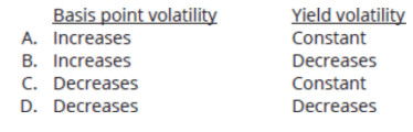
Q1. Which of the following choices correctly characterizes basis point volatility and yield volatility as a function of the level of the rate within the lognormal model?

Practice Questions: Q1 Answer

Explanation: A is correct.

Choices B and D can be eliminated because yield volatility is constant. Basis point volatility under the CIR model increases at a decreasing rate, whereas basis point volatility under the lognormal model increases linearly. Therefore, basis point volatility is an increasing function for both models.

Topic 3. Terminal Distributions for Normal, CIR and Lognormal Models

Fig 15.1 illustrates the terminal distribution for short-term rates for normal, CIR, and lognormal models after 10 years
- With equal means and standard deviations, the normal model shows a positive probability of negative interest rates.
- Longer forecast horizons increase the chance of negative rates in the normal model.
- The left tail of the normal distribution lies above zero for negative rates, highlighting a key drawback.
- Unlike the normal distribution, lognormal and CIR distributions are always non-negative and right-skewed. This significantly affects pricing, especially for out-of-the-money options.

Practice Questions: Q2

Q2. Which of the following statements is most likely a disadvantage of the CIR model?

A. Interest rates are always non-negative.

B. Option prices from the CIR distribution may differ significantly from lognormal or normal distributions.

C. Basis point volatility increases during periods of high inflation.

D. Long-run interest rates hover around a mean-reverting level.

Practice Questions: Q2 Answer

Explanation: B is correct.

Choices A and C are advantages of the CIR model. Out-of-the money option prices may differ with the use of normal or lognormal distributions.

Topic 4. Lognormal Model with Deterministic Drift

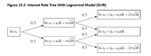
Lognormal Model with Deterministic Drift: $d [ln (r)] = a (t) d t + σ d w$ .
- The natural log of the short-term rate follows a normal distribution.
- This model can be used to construct an interest rate tree (similar to Ho-Lee, where drift can vary), as shown in Fig 15.2

Topic 4. Lognormal Model with Deterministic Drift

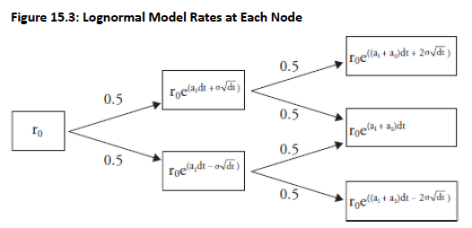
If each node in Figure 15.3 is exponentiated, the tree will display the interest rates at each node. For example, the adjusted period 1 upper node would be calculated as:
Unlike Ho-Lee model where the drift terms are additive, the drift terms in the lognormal model are multiplicative.
The implication is that all rates in the tree will always be positive since for all x.
Also, since and if we assume and then Hence, volatility is a percentage of the rate.
For example, if σ = 20%, then the rate in the upper node will be 20% above the current short-term rate.

\exp \left(\ln r_0+a_1 d t+\sigma \sqrt{d t}\right)=r_0 e^{\left(a_1 d t+\sigma \sqrt{d t}\right)}

e^x >0

\mathrm{e}^{\mathrm{x}} \approx 1+\mathrm{x},

a_1=0

dt=1,

r_0 e^\sigma \approx r_0(1+\sigma).

Practice Questions: Q3

Q3. Which of the following statements best characterizes the differences between the Ho-Lee model with drift and the lognormal model with drift?

A. In the Ho-Lee model and the lognormal model the drift terms are multiplicative.

B. In the Ho-Lee model and the lognormal model the drift terms are additive.

C. In the Ho-Lee model the drift terms are multiplicative, but in the lognormal model the drift terms are additive.

D. In the Ho-Lee model the drift terms are additive, but in the lognormal model the drift terms are multiplicative.

Practice Questions: Q3 Answer

Explanation: D is correct.

The Ho-Lee model with drift is very flexible, allowing the drift terms each period to vary. Hence, the cumulative effect is additive. In contrast, the lognormal model with drift allows the drift terms to vary, but the cumulative effect is multiplicative.

Topic 4. Lognormal Model With Mean Reversion

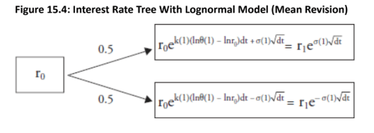
Black-Karasinski model: The combination of a lognormal distribution and a mean-reverting process.
This model offers flexibility by allowing for time-varying volatility and mean reversion.
In logarithmic terms, the model is: $d [ln (r)] = k (t) [ln θ (t) - ln (r)] d t + σ (t) d w$ .
- The natural log of the short-term rate follows a normal distribution and reverts to the long-run mean of $ln [θ (t)]$ based on the adjustment parameter $k (t)$
- Volatility is time-dependent, making the Vasicek model time-varying.
Interest Rate Tree Characteristics: The interest rate tree for this model is more complex but retains a basic structure similar to previous models.
- It does not produce a naturally recombining interest rate tree.
- To force the tree to recombine, the time steps ( $d t$ ) must be recalibrated. For example,

k(2)=\frac{1}{d t_2}\left[1-\frac{\sigma(2) \sqrt{d t_2}}{\sigma(1) \sqrt{d t_1}}\right] .

Practice Questions: Q4

Q4. Which of the following statements is true regarding the Black-Karasinski model?

A. The model produces an interest rate tree that is recombining by definition.

B. The model produces an interest rate tree that is recombining when the dt variable is manipulated.

C. The model is time-varying and mean-reverting with a slow speed of adjustment.

D. The model is time-varying and mean-reverting with a fast speed of adjustment.

Practice Questions: Q4 Answer

Explanation: B is correct.

A feature of the time-varying, mean-reverting lognormal model is that it will not recombine naturally. Rather, the time intervals between interest rate changes are recalibrated to force the nodes to recombine. The generic model makes no prediction on the speed of the mean reversion adjustment.