Book 1. Market Risk
FRM Part 2
MR 8. Correlation Basics
Presented by: Sudhanshu
Module 1. Financial Correlation Risk
Module 2. Correlation Swaps, Risk Management and The Global Financial Crisis
Module 3. Role of Correlation Risk in Other Types of Risks
Module 1. Financial Correlation Risk
Topic 1. Financial Correlation Risk
Topic 2. Categories of Financial Correlation
Topic 3. Correlation Risk in Credit Default Swap
Topic 4. Correlations in Financial Investments
Topic 5. Correlations and Risk-Adjusted Returns
Topic 6. Correlation Options
Topic 7. Exchange Option and Quanto Option
Topic 8. Quanto Option: Example

Topic 1. Financial Correlation Risk
-
Correlation risk measures the risk of financial loss resulting from adverse changes in correlations between financial or nonfinancial assets.
-
This risk appears in five common finance areas: (1) investments, (2) trading, (3) risk management, (4) global markets, and (5) regulation.
-
Examples of Financial Correlation Risk
-
Interest Rates and Commodities: A negative correlation between interest rates and commodity prices means that if interest rates rise, losses occur in commodity investments.
-
The 2007–2009 Financial Crisis: The crisis illustrated the global impact of this risk, as assets that previously had very low or negative correlations suddenly became highly positively correlated and fell in value together across global markets.
-
Structured Products: Correlation risk is a growing concern in structured products like Credit Default Swaps (CDSs), Collateralized Debt Obligations (CDOs), multi-asset correlation options, and correlation swaps.
-
-
Financial correlations can be categorized as static or dynamic:
| Category | Definition | Examples |
|---|---|---|
| Static | Do not change and measure the relationship between assets for a specific time period. | Value at Risk (VaR), copula correlations for CDOs, and the binomial default correlation model. |
| Dynamic | Measure the comovement of assets over time. | Pairs trading, deterministic correlation approaches, and stochastic correlation processes. |
Topic 2. Categories of Financial Correlation
Practice Questions: Q1
Q1. Which of the following measures is most likely an example of a dynamic financial correlation measure?
A. Pairs trading.
B. Value at risk (VaR).
C. Binomial default correlation model.
D. Copula correlations for collateralized debt obligations (CDOs).
Practice Questions: Q1 Answer
Explanation: A is correct.
Dynamic financial correlations measure the comovement of assets over time. Examples of dynamic financial correlations are pairs trading, deterministic correlation approaches, and stochastic correlation processes. The other choices are examples of static financial correlations.
-
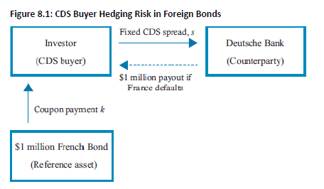
CDS Valuation: A CDS spread is valued based on the default probability of the reference asset (e.g., a French bond) and the joint default correlation of the counterparty (CDS seller) and the reference asset.
-
Wrong-Way Risk (WWR): If a positive correlation exists between the reference asset and the counterparty, the investor has WWR. A high correlation risk increases the probability that both the reference asset and the counterparty will default, which is the worst-case scenario for the investor, leading to a loss of the entire investment.
-
Impact on Spread: The higher the correlation risk, the lower the CDS spread. This relationship, however, may be nonmonotonous, meaning the spread can sometimes increase or decrease as correlation risk rises, particularly in cases of high negative correlation.
Topic 3. Correlation Risk in Credit Default Swap
Topic 4. Correlations in Financial Investments
-
Modern Portfolio Theory: Harry Markowitz provided the foundation of modern investment theory in 1952 by demonstrating the role correlation plays in reducing risk through diversification.
- Portfolio Calculations: The portfolio's expected return (μP) is the weighted average of the individual asset returns, while the risk (σP) or standard deviation) is determined by the variances, weights, and the covariance between assets.
- Portfolio Mean Return (Two Assets):
-
Portfolio Standard Deviation/Risk (2 Assets):
-
Covariance: A measure of how two assets move together over time, capturing both the magnitude and direction of movement.
-
-
-
Correlation Coefficient (ρXY): Standardizes the comovement (covariance) between assets.
-
-
-
Markowitz emphasized the importance of risk-adjusted returns, often measured by the Return/Risk ratio
-
Inverse Relationship: The lower the correlation between two assets, the higher the Return/Risk ratio.
- A very high negative correlation (e.g., -0.9) results in a high Return/Risk ratio.
- A very high positive correlation (e.g., +0.9) results in a low Return/Risk ratio.
Topic 5. Correlations and Risk-Adjusted Returns

Topic 6. Correlation Options
-
General Characteristics
-
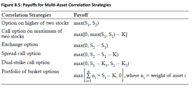
Correlation options have prices that are highly sensitive to the correlation between two or more assets and are often referred to as multi-asset options.
-
Pricing Rule: For most multi-asset correlation strategies, a lower correlation results in a higher option price. This is because a low correlation increases the chance of one asset price going higher while the other is lower, which improves the probability of a high payout.
-
Exception: The only correlation strategy where a lower correlation is not desirable (it reduces the option price) is the option on the worse of two stocks, which has a payoff equal to the minimum of the two stock prices, max(0, min(S1,S2)−K). This is not listed in Fig 8.5
-
-
Exchange Option
- .The buyer has the right to receive asset 2 and give away asset 2 at maturity.
-
Implied Volatility ( ) : The option's implied volatility, which is a major factor in its price, is highly sensitive to correlation (covariance).
- Correlation Impact: The exchange option price increases as the correlation between the two assets decreases, because a lower correlation makes a large spread (S2−S1) more likely. The price of the exchange option is close to zero when the correlation is close to 1.
-
Quanto Option
- Purpose: The quanto option is designed to protect a domestic investor from foreign currency risk.
-
Structure: It sets a fixed currency exchange rate for converting foreign currency profits into the domestic currency upon exercise.
-
Correlation Impact: Lower correlations between currencies result in higher prices for quanto options. If the foreign asset (e.g., Nikkei index) increases but the foreign currency (e.g., Yen) decreases, the financial institution selling the option will require more of the foreign currency to convert the investor's profits at the fixed rate, increasing the option's cost.
Topic 7. Exchange Option and Quanto Option
-
Example: Suppose a U.S. investor buys a quanto call to invest in the Nikkei index and protect potential gains by setting a fixed currency exchange rate (USD per JPY). How does the correlation between the call on the Nikkei index and the exchange rate impact the price of the quanto option?
-
Answer: The U.S. investor buys a quanto call on the Nikkei index that has a fixed exchange rate for converting yen to dollars. If the correlation coefficient is positive (negative) between the Nikkei index and the yen relative to the dollar, an increasing Nikkei index results in an increasing (decreasing) value of the yen. Thus, the lower the correlation, the higher the price for the quanto option. If the Nikkei index increases and the yen decreases, the financial institution will need more yen to convert the profits in yen from the Nikkei investment into dollars.
Topic 8. Quanto Option: Example
Module 2. Correlation Swaps, Risk Management and The Global Financial Crisis
Topic 1. Correlation Swaps
Topic 2. Correlation Swap Example
Topic 3. Alternative Ways to Trade Correlation
Topic 4. Relationship Between VaR and Correlation
Topic 5. Factors Contributing to the Global Financial Crisis (GFC)
Topic 6. Market Collapse and Correlation Breakdown During the GFC
Topic 7. Regulatory Response and New Risk Models
Topic 1. Correlation Swaps
-
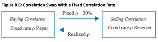
A correlation swap is a derivative contract used to trade a fixed correlation between two or more assets with the correlation that is actually realized over the life of the swap (the realized or stochastic correlation).
-
In a typical swap structure, the party buying the correlation swap pays a fixed correlation rate (ρfixed) and receives the realized correlation (ρrealized). The party selling the swap receives the fixed rate and pays the realized correlation.
-
Payoff Calculation
-
The present value of the correlation swap increases for the correlation buyer if the realized correlation increases.
-
The realized correlation for a portfolio of n assets is calculated by averaging all pairwise correlation coefficients (ρi,j):
-
-
-
The payoff for the investor buying the correlation swap is calculated as:
-
-
-
Topic 2. Correlation Swap Example
-
Suppose a correlation swap buyer pays a fixed correlation rate of 0.2 with a notional value of $1 million for one year for a portfolio of three assets. The realized pairwise correlations of the daily log returns [ln(St/St-1)] at maturity for the three assets are ρ2,1=0.6, ρ3,1=0.2 and ρ3,2=0.04. (Note that for all pairs i > j.) What is the correlation swap buyer’s payoff?
-
Solution: The realized correlation is calculated as:
-
-
-
-
The payoff for the correlation swap buyer is then calculated as:
-
$1,000,000 × (0.28 − 0.20) = $80,000
-
Practice Questions: Q1
Q1. Suppose an individual buys a correlation swap with a fixed correlation of 0.2 and a notional value of $1 million for one year. The realized pairwise correlations of the daily log returns at maturity for three assets are What is the correlation swap buyer’s payoff at maturity?
A. $100,000.
B. $200,000.
C. $300,000.
D. $400,000.
Practice Questions: Q1 Answer
Explanation: B is correct.
First, calculate the realized correlation as follows:
The payoff for the correlation buyer is then calculated as:
-
Investors can also effectively "buy" or "sell" correlation using other derivatives:
-
Buying Correlation using Options: Buy call options on a stock index (e.g., S&P 500) and sell call options on individual stocks within the index. If correlation increases, the implied volatility and price of the index call options are expected to increase more than the prices of the individual stock options.
-
Buying Correlation using Swaps: Pay fixed in a variance swap on an index and receive fixed on individual securities within the index. An increase in correlation causes the index variance to increase, which increases the value of the position for the fixed variance swap payer.
-
Topic 3. Alternative Ways to Trade Correlation
Topic 4. Relationship between VaR and Correlation
-
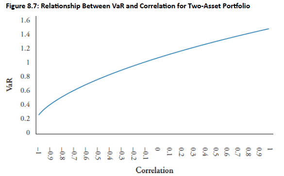
The VaR is calculated using the variance-covariance (delta-normal) method as:
-
where : Daily portfolio volatility, α: Z-value and x: Number of trading day
-
-
The portfolio volatility is defined as:
- where C: returns covariance matrix, and βh,βv: horizontal and vertical vectors of investment amount
- Relationship: The VaR for a portfolio increases as the correlation between the two assets increases. This is because higher correlation reduces the benefits of diversification.
-
The BCBS requires banks to hold capital for assets in the trading book of at least three times greater than 10-day VaR.
Practice Questions: Q2
Q2. Suppose a financial institution has a two-asset portfolio with $7 million in asset A and $5 million in asset B. The portfolio correlation is 0.4, and the daily standard deviation of returns for asset A and B are 2% and 1%, respectively. What is the 10-day value at risk (VaR) of this portfolio at a 99% confidence level (α = 2.33)?
A. $1.226 million.
B. $1.670 million.
C. $2.810 million.
D. $3.243 million.
Practice Questions: Q2 Answer
Explanation: A is correct.
The first step in solving for the 10-day VaR requires calculating the covariance matrix.
Thus, the covariance matrix, C, can be represented as:
Next, the standard deviation of the portfolio, , is determined as follows:
Step 1: Compute
Step 2: Compute
Step 3: Compute :
The 10-day portfolio VaR (in millions) at the 99% confidence level is then computed as:
Topic 5. Factors Contributing to the Global Financial Crisis (GFC)
- The financial crisis resulted from a combination of high asset correlations, an overly optimistic housing market, excessive leverage, and inadequate risk management across sectors and regions.
- Following the internet bubble, a low-rate environment with declining credit spreads and volatility encouraged risk-taking, while borrowers overextended on overvalued properties fueled by liberal lending policies.
- New structured products like collateralized debt obligations (CDOs), constant-proportion debt obligations (CPDOs), and credit default swaps (CDSs) facilitated real estate speculation without proper oversight from rating agencies, risk managers, or regulators.
- Risk managers misapplied the copula correlation model to CDOs containing up to 125 assets, requiring management of 7,750 correlations [125 × 124 / 2] that were not properly understood or measured.
- Large hedge funds employed strategies of being long the equity tranche (first 3% of defaults) and short the mezzanine tranche (3%-7% of defaults), believing correlations across tranches provided hedging, which ultimately led to massive losses and bankruptcies.
Topic 6. Market Collapse and Correlation Breakdown During the GFC
- The CDO market exploded from $64 billion in 2003 to $455 billion in 2006, primarily driven by residential mortgages, while the CDS market grew from $8 trillion to $60 trillion between 2004 and 2007.
- When General Motors and Ford were downgraded to junk status in May 2005, equity tranche spreads increased dramatically while mezzanine tranche spreads decreased, causing losses on both sides of hedge fund positions due to misunderstood correlation dynamics.
- Housing price stagnation in 2006 triggered the first wave of subprime mortgage defaults, which escalated into a full real estate market collapse in 2007, spreading globally as stock and commodity markets crashed with sharply increased correlations.
- Default rates rose so dramatically that all CDO tranches lost value simultaneously, with even AAA-rated senior tranches losing 20% of their value, while leverage ratios of 10-20 times magnified losses across the system.
- Major institutions failed due to excessive leverage and counterparty exposure, including AIG's $500 billion in CDS exposure with minimal reinsurance and Lehman Brothers' 30.7x leverage ratio with 8,000 derivative counterparties at bankruptcy.
Topic 7. Regulatory Response and New Risk Models
- Regulators developed Basel III standards in response to the crisis, implementing new requirements for liquidity ratios, leverage ratios, and capital buffers for financial institutions.
- New correlation models are being developed and implemented to address the failures of the original copula model, including the Gaussian copula, credit value adjustment (CVA) for derivatives correlations, and wrong-way risk (WWR) correlation measures.
- These enhanced models aim to better capture correlated defaults in multi-asset portfolios and prevent the systematic underestimation of tail risk that contributed to the financial crisis.
Practice Questions: Q3
Q3. In May of 2005, several large hedge funds had speculative positions in the collateralized debt obligations (CDOs) tranches. These hedge funds were forced into bankruptcy due to the lack of understanding of correlations across tranches. Which of the following statements best describe the positions held by hedge funds at this time and the role of changing correlations? Hedge funds held a:
A. long equity tranche and short mezzanine tranche when the correlations in both tranches decreased.
B. short equity tranche and long mezzanine tranche when the correlations in both tranches increased.
C. short senior tranche and long mezzanine tranche when the correlation in the mezzanine tranche increased.
D. long mezzanine tranche and short equity tranche when the correlation in the mezzanine tranche decreased.
Practice Questions: Q3 Answer
Explanation: A is correct.
A number of large hedge funds were long the CDO equity tranche and short the CDO mezzanine tranche. Following the change in bond ratings for Ford and General Motors, the equity tranche spread increased. This caused losses on the long equity tranche position. At the same time, the mezzanine tranche spread decreased, which led to losses on the short mezzanine tranche position.
Module 3. Role of Correlation Risk in Other Types of Risks
Topic 1. Role of Correlation Risk in Market Risk
Topic 2. Role of Correlation Risk in Credit Risk
Topic 3. Role of Correlation Risk in Systemic Risk
Topic 4. Role of Correlation Risk in Concentration Risk
Topic 5. Example 1: Concentration Ratio for Bank X and One Loan to Company A
Topic 6. Example 1: Concentration Ratio for Bank Y and Two Loans to Companies A and B
Topic 7. Example 1: Concentration Ratio for Bank Y and Three Loans to Company A, B and C
Topic 1. Role of Correlation Risk in Market Risk
- Risk managers must understand the relationship between correlation risk and other risk types, including market, credit, systemic, and concentration risk.
- Market risk encompasses interest rate risk, currency risk, equity price risk, and commodity risk, and is typically measured using Value at Risk (VaR).
- The covariance matrix of assets is a critical input for VaR calculations, making correlation risk extremely important for accurate market risk measurement.
- Expected shortfall (ES) quantifies market risk for extreme events or tail risk scenarios, complementing VaR by capturing the magnitude of losses beyond the VaR threshold.
- Correlation risk—the risk that correlations between assets change over time—directly impacts the stability and accuracy of the covariance matrix used in VaR and ES calculations as market conditions evolve.
Topic 2. Role of Correlation Risk in Credit Risk
- Risk managers measure credit risk through migration risk (the risk of credit rating downgrades that increase default probabilities and decrease asset values) and default risk.
- Correlation between a reference asset and its counterparty (such as a CDS seller) is critical, as higher correlation increases the probability of total investment loss.
- Default correlation quantifies the degree to which defaults occur simultaneously across a portfolio, with lower correlations indicating greater diversification and reduced credit risk for financial institutions.
- Empirical studies show most default correlations across industries are positive, except for the energy sector, which exhibits little to no correlation with other sectors and greater recession resistance.
- Default correlations within industries are significantly higher than across industries, indicating that systematic market factors drive defaults more than company-specific factors (e.g., Chrysler's default increases Ford and GM's default likelihood rather than benefiting them).
- Commercial banks limit industry-specific exposures and diversify across industries to lower portfolio default correlations and reduce concentration risk.
Topic 2. Role of Correlation Risk in Credit Risk
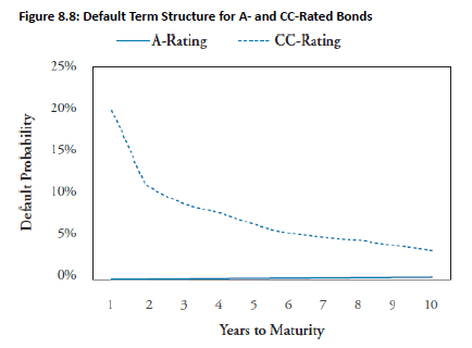
- The term structure of defaults shows that investment-grade bonds have slightly increasing default probabilities over time. This is expected because bonds are more likely to default as many market or company factors can change over a longer time period.
- Non-investment grade bonds exhibit higher near-term default risk that decreases if the company survives its immediate distressed situation.
Practice Questions: Q1
Q1. Suppose a creditor makes a $4 million loan to Company X and a $4 million loan to Company Y. Based on historical information of companies in this industry, Companies X and Y each have a 7% default probability and a default correlation coefficient of 0.6. The expected loss for this creditor under the worst-case scenario assuming loss given default is 100% is closest to:
A. $280,150.
B. $351,680.
C. $439,600.
D. $560,430.
Practice Questions: Q1 Answer
Explanation: B is correct.
The worst-case scenario is the joint probability that both loans default at the same time. The joint probability of default is computed as:
Thus, the expected loss for the worst-case scenario for the creditor is:
Practice Questions: Q2
Q2. The relationship of correlation risk to credit risk is an important area of concern for risk managers. Which of the following statements regarding default probabilities and default correlations is incorrect?
A. Creditors benefit by diversifying exposure across industries to lower the default correlations of debtors.
B. The default term structure increases with time to maturity for most investment grade bonds.
C. The probability of default is higher in the long-term time horizon for non-investment grade bonds.
D. Changes in the concentration ratio are directly related to changes in default correlations.
Practice Questions: Q2 Answer
Explanation: C is correct.
The probability of default is higher in the immediate time horizon for noninvestment grade bonds. The probability of default decreases over time if the company survives the near-term distressed situation.
- Lehman Brothers' bankruptcy in September 2008 signaled the severity of the financial crisis and highlighted systemic risk—the potential collapse of the entire financial system.
- From October 2007 to March 2009, the Dow Jones Industrial Average fell over 50%, with only 11 of 500 stocks in the S&P 500 Index gaining value, reflecting widespread economic impact including decreased disposable income, lower GDP, and rising unemployment.
- The 11 stocks that increased were concentrated in recession-resistant sectors: consumer staples (Family Dollar, Ross Stores, Walmart), education (Apollo Group, DeVry), pharmaceuticals (Edward Lifesciences, Gilead), agriculture (CF Industries), entertainment (Netflix), energy (Southwestern Energy), and automotive (AutoZone).
- During the August 2008 to March 2009 freefall, stock correlations increased dramatically from a pre-crisis average of 27% to over 50%, causing diversification benefits to disappear precisely when investors needed them most.
- The severity of correlation risk during systemic crises is amplified by higher correlations not only among U.S. equities but also between U.S. equities, bonds, and international equities, eliminating traditional diversification strategies across asset classes.
Topic 3. Role of Correlation Risk in Systemic Risk
- Concentration risk represents the financial loss arising from exposure to multiple counterparties within a specific group, measured by the concentration ratio.
- A lower concentration ratio indicates more diversified default risk; for example, a creditor with 100 equal-sized loans to different entities has a concentration ratio of 0.01 (1/100), while a single loan results in a ratio of 1.0.
- Loans can be analyzed by grouping them into sectors, where higher default correlations within sectors increase the likelihood that multiple loans will default simultaneously when one loan defaults.
- When loan defaults are more highly correlated within specific sectors, concentration risk intensifies as correlated defaults reduce the benefits of diversification.
- The relationship between concentration risk and correlation risk is critical, as higher correlations within concentrated exposures can amplify portfolio losses during adverse events.
Topic 4. Role of Correlation Risk in Concentration Risk
- Example: Suppose Commercial Bank X makes a $5 million loan to Company A, which has a 5% default probability. What is the concentration ratio and expected loss (EL) for Commercial Bank X under the worst-case scenario? Assume loss given default (LGD) is 100%.
- Answer: Commercial Bank X has a concentration ratio of 1.0 because there is only one loan. The worst-case scenario is that Company A defaults resulting in a total loss of loan value. Given that there is a 5% probability that Company A defaults, EL for Commercial Bank X is $250,000 (= 0.05 × 5,000,000).
Topic 5. Example 1: Concentration Ratio for Bank X and One Loan to Company A
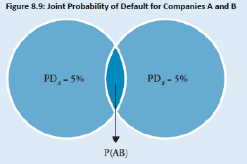
- Example: Suppose Commercial Bank Y makes a $2,500,000 loan to Company A and a $2,500,000 loan to Company B. Assuming Companies A and B each have a 5% default probability, what is the concentration ratio and expected loss (EL) for Commercial Bank Y under the worst-case scenario? Assume default correlation between companies is 1.0 and loss given default (LGD) is 100%.
- Answer: Commercial Bank Y has a concentration ratio of 0.5 (calculated as 1/2). The expected loss for Commercial Bank Y depends on the default correlation of Companies A and B. Note that changes in the concentration ratio are directly related to changes in the default correlations. A decrease in the concentration ratio results in a decrease in the default correlation. The default of Companies A and B can be expressed as two binomial events with a value of 1 in default and 0 if not in default. Figure 8.9 illustrates the joint probability that both Companies A and B are in default, P(AB).
Topic 6. Example 2: Concentration Ratio for Bank Y and Two Loans to Companies A and B
-
The following equation computes the joint probability that both Companies A and B are in default at the same time:
-
-
If the default correlation between Companies A and B is 1.0, the expected loss for Commercial Bank Y is $250,000 (0.05 × $5,000,000). Notice that when the default correlation is 1.0, this is the same as making a $5 million loan to one company.
-
Now, let’s assume that the default correlation between Companies A and B is 0.5. What is the expected loss for Commercial Bank Y? The joint probability of default for A and B, assuming a default correlation of 0.5, is:
-
-
Thus, the expected loss for the worst-case scenario for Commercial Bank Y is:
-
EL = 0.02627 × $5,000,000 = $131,350
-
-
If we assume the default correlation coefficient is 0, the joint probability of default is 0.0025 and the expected loss for Commercial Bank Y is only $12,500. Thus, a lower default correlation results in a lower expected loss under the worst-case scenario.
Topic 6. Example 2: Concentration Ratio for Bank Y and Two Loans to Companies A and B
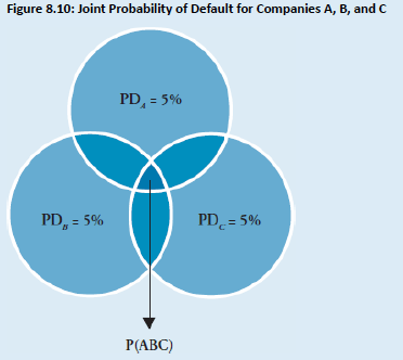
- Example: Now we can examine what happens to the joint probability of default (i.e., the worst-case scenario) if the concentration ratio is reduced further. Suppose that Commercial Bank Z makes three $1,666,667 loans to Companies A, B, and C. Also assume the default probability for each company is 5%. What is the concentration ratio for Commercial Bank Z, and how will the joint probability be impacted?
- Answer: Commercial Bank Z has a concentration ratio of 0.333 (calculated as 1/3). Figure 8.10 illustrates the joint probability of all three loans defaulting at the same time, P(ABC) (i.e., the small area in the center of Figure 8.10 where all three default probabilities overlap). Note that as the concentration ratio decreases, the joint probability also decreases.
Topic 7. Example 3: Concentration Ratio for Bank Z and Two Loans to Companies A, B and C