Book 2. Quantitative Analysis
FRM Part 1
QA 13. Simulation and Bootstrapping
Presented by: Sudhanshu
Module 1. Monte-Carlo Simulation and Sampling Error Reduction
Module 2. Bootstrapping and Random Number Generation
Module 1. Monte-Carlo Simulation and Sampling Error Reduction

Topic 1. Introduction to Simulation and Bootstrapping
Topic 2. Steps in Monte Carlo Simulation
Topic 3. Monte Carlo Sampling Error & Its Reduction
Topic 4. Antithetic Variates Method
Topic 5. Control Variates Method
Topic 1. Introduction to Simulation and Bootstrapping
- Simulation is a statistical technique to model uncertainty in complex systems.
- Monte Carlo Simulation (MCS): Uses random numbers from theoretical distributions to simulate possible outcomes.
- Bootstrapping: Uses historical data instead of assumptions about distributions.
-
Applications in Finance:
- Valuation of exotic derivatives
- Risk estimation under macroeconomic stress
- Regulatory capital projections
Practice Questions: Q1
Q1. Which of the following statements regarding Monte Carlo simulation is least accurate? When using Monte Carlo simulation:
A. simulated data is used to numerically approximate the expected value of a function.
B. the user specifies a complete data generating process (DGP) that is used to produce simulated data.
C. the observed data are used directly to generate a simulated data set.
D. a full statistical model is used that includes an assumption about the distribution of the shocks.
Practice Questions: Q1 Answer
Explanation: C is correct.
In both Monte Carlo simulation and bootstrapping, the goal is to numerically approximate the expected value of a complex function through the use of computer-generated values (i.e., simulated data). The main difference between Monte Carlo simulation and bootstrapping is the source of the simulated data: in Monte Carlo simulation, the user specifies a complete DGP that is used to produce
the simulated data, while in bootstrapping, the observed data are used directly to generate the simulated data set- without specifying a complete DGP.
Topic 2. Steps in Monte Carlo Simulation
-
Five Key Steps:
- Generate random inputs from an assumed data-generating process (DGP).
- Compute statistic of interest .
- Repeat the above steps N times to form
- Estimate quantity of interest using the replicated outputs.
- Evaluate the accuracy by estimating the standard error:
- Common distributions used: Normal, t-distribution
- Output: Distribution of the estimate instead of a single value
-
Example: Estimating ending capital of a portfolio:
Topic 3. Monte Carlo Sampling Error & Its Reduction
- Sampling Error: Occurs due to limited number of simulations (N)
- Formula:
-
-
Increasing N improves accuracy:
- 4×N → SE reduced by 2×
- 100×N → SE reduced by 10×
-
Increasing N improves accuracy:
-
Illustration:
- Note 1: We cannot control the standard deviation
- Note 2: Increasing number of simulations is costly from computational perspective
- Sampling error can also be reduced by variance reduction techniques
- Two most techniques for variance reduction are antithetic variates and control variates
Practice Questions: Q2
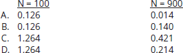
Q2. Suppose an analyst is concerned about Monte Carlo sampling error. Based on an initial Monte Carlo simulation with 100 replications, the results indicated a standard deviation of 12.64. The simulation was rerun with 900 replications and the standard
deviation remained at 12.64. What are the standard error estimates for the simulations with 100 replications and 900 replications, respectively?
Practice Questions: Q2 Answer
Explanation: C is correct.
The standard error is determined by dividing the standard deviation by the square root of the number of replications The standard error estimate for the first simulation of 100 replications is 1.264 (i.e., 12.64/ 10). With 900 replications, the standard error estimate is reduced to 0.4213 (i.e., 12.64/ 30).
Topic 4. Antithetic Variates Method
- Goal: Reduce variance by pairing each simulation with its negative counterpart.
- Random input set:
- Antithetic pair:
- Perfect negative correlation: Corr(ut,−ut)=−1\text{Corr}(u_t, -u_t) = -1−ut-u_t
-
Mechanism:
- Generate x1,x2x_1, x_2x1,x2 → compute average:
-
Reduces variance due to negative covariance.
-
- Used when full sampling range is expensive to generate.
Topic 5. Control Variates Method
- Use of a known variable yyy (control) to reduce error in estimating unknown xxx.
- New estimator:
- Effective when:
-
This technique is effective only if:
- This can also be expressed as:
- Alternately,
- Example: Pricing Asian options using European option (with known Black-Scholes price) as control:
Practice Questions: Q3
Q3. A concern for Monte Carlo simulations is the size of the sampling error. One way to reduce the sampling error is to use the antithetic variate technique. Which of the following statements best describes this technique?
A. The simulation is rerun using a complement set of the original set of random variables.
B. The number of replications is increased significantly to reduce sampling error.
C. Sample data is replaced after every replication to ensure it has an equal probability of being redrawn.
D. The data generating process (DGP) is approximated by redefining the unknown variable with a variable that has known properties.
Practice Questions: Q3 Answer
Explanation: A is correct.
The antithetic variate technique reduces Monte Carlo sampling error by rerunning the simulation using a complement set of the original set of random variables.
Module 2. Bootstrapping and Random Number Generation
Topic 1. Bootstrapping Method & Comparison with MCS
Topic 2. When Bootstrapping Fails
Topic 3. Pseudo-Random Number Generation
Topic 4. Disadvantages of Simulation
Topic 1. Bootstrapping Method & Comparison with MCS
- Draws samples with replacement from historical data
- Doesn’t assume any parametric distribution
-
Two types:
- i.i.d. Bootstrapping: Assumes data independence; randomly draws from full data
- CBB (Circular Block Bootstrapping): Maintains time dependency by sampling blocks
- Example of i.i.d.: From 10 observations → Sample 3 with replacement: {x2, x7, x9}, etc.
-
Example of CBB: 10 blocks of 3 consecutive data points:
-
Practice Questions: Q4
Q4. Which of the following statements regarding the bootstrapping method is least accurate? Bootstrapping simulations:
A. draw data from historical data sets.
B. replace drawn data so it can be redrawn.
C. require assumptions with respect to the true distribution of the parameter estimates.
D. rely on the key assumption that the present resembles the past.
Practice Questions: Q4 Answer
Explanation: C is correct.
The bootstrapping technique does not require any assumptions with respect to the true distribution of the parameter estimates. Bootstrapping simulations repeatedly draw data from historical data sets, and then replace the data so it can be redrawn. The bootstrapping method is only as valid as the assumption that the
present resembles the past.
Topic 2. When Bootstrapping Fails
-
Situations Where Bootstrapping Is Ineffective
-
Complete Dataset is Non-Reliable
- Bootstrapping assumes that past data reflects the future.
- If market conditions today are abnormal, bootstrapped results may mislead.
- Example: During the 2007–2009 financial crisis, using bootstrapping on low-volatility pre-crisis data would understate the risk (e.g., Value-at-Risk or VaR estimates too low).
-
Structural Market Changes
- When permanent shifts in market conditions occur, past data becomes irrelevant.
-
Example:
- U.S. T-bill rates remained near zero for a decade post-2008, a condition never seen in historical data.
- Bootstrapping pre-2008 data would fail to replicate post-2008 reality.
-
Complete Dataset is Non-Reliable
Practice Questions: Q5
Q5. The bootstrapping method is most likely to be effective when the:
A. data contains outliers.
B. present is different from the past.
C. data is independent.
D. markets have experienced structural changes.
Practice Questions: Q5 Answer
Explanation: C is correct.
The bootstrapping method is most likely to be effective when the data is independent and there are no outliers in the data. Bootstrapping uses the entire data set to generate a simulated sample, so the bootstrapping method should be reliable if the current state of the financial market is the same as its normal state, meaning that no structural changes have taken place.
Topic 3. Pseudo-Random Number Generation
-
What Are Pseudo-Random Number Generators (PRNGs)?
-
Random number generators are used to produce an irregular sequence of numerical values.
- Pseudo-Random Number Generators (PRNGs): Algorithms that simulate random sequences using mathematical formulas.
- Not truly random, but appear random for practical purposes. They produce numbers in the uniform (0,1) interval.
-
- Key Term: Seed Value – Starting input to the PRNG. The same seed always produces the same sequence.
-
Benefits of PRNG in Finance
-
Repeatability
- Ideal for testing multiple models under identical simulated conditions.
- Regulators may require simulations to be reproduced for audit or validation.
-
Computing Clusters
- Large simulations (e.g., thousands of financial instruments) can be run on computing clusters.
- Using the same seed across clusters ensures synchronized scenarios.
- Control Over Simulation Inputs: Enables comparison of strategies under identical “random” paths.
-
Repeatability
Practice Questions: Q6
Q6. Which of the following statements regarding the pseudo-random number generation method is least accurate? Pseudo-random numbers are:
A. not truly random.
B. actually generated from a formula.
C. determined by the choice of the initial seed value.
D. impossible to predict.
Practice Questions: Q6 Answer
Explanation: D is correct.
Pseudo-random numbers appear random because they are difficult to predict. However, they are produced by deterministic functions that are complex rather than truly random. The initial choice of a seed value determines the series of random numbers that is generated.
-
Data Generating Process (DGP) Specification
- Unrealistic assumptions about model inputs can lead to imprecise results
- Different DGP assumptions may produce substantially different outcomes
-
Common misspecification: assuming normal distribution for fat-tailed data.
- Example: Option prices are typically fat-tailed, not normally distributed
- Results remain inaccurate regardless of number of replications
-
Computational Cost
- Large number of replications needed to reduce variation (≥10,000 typical)
- Complex parameters require extremely long computation times
- Market complexity continues to increase despite processor improvements
- High computational costs may limit practical application
Topic 4. Disadvantages of Simulation Approach
Practice Questions: Q7
Q7. Monte Carlo simulation is a widely used technique in solving economic and financial problems. Which of the following statements is least likely to represent a limitation of the Monte Carlo technique when solving problems of this nature?
A. High computational costs arise with complex problems.
B. Simulation results are experiment-specific because financial problems are
analyzed based on a specific data generating process (DGP) and set of equations.
C. Results of most Monte Carlo experiments are difficult to replicate.
D. If the input variables have fat tails, Monte Carlo simulation is not relevant
because it always draws random variables from a normally distributed population.
Practice Questions: Q7 Answer
Explanation: D is correct.
A disadvantage of Monte Carlo simulations is that imprecise results may occur when the assumptions of model inputs or DGP are unrealistic. The distribution of input variables does not need to be the normal distribution. Problems will arise if a real-world variable is fat-tailed, but the model erroneously draws option prices from a normal distribution.