Book 2. Quantitative Analysis
FRM Part 1
QA 15. Machine Learning and Prediction
Presented by: Sudhanshu
Module 1. Categorical Variables, Regularization and Logistic Regression
Module 2. Decision Trees, Ensemble Learning, K-Nearest Neighbors and Support Vector Machines
Module 3. Neural Networks and Model Performance
Module 1. Categorical Variables, Regularization and Logistic Regression

Topic 1. Categorical Variables
Topic 2. Regularization
Topic 3. Ridge Regression (L2 Regularization)
Topic 4. LASSO (L1 Regularization)
Topic 5. Logistic Regression
Topic 6. Logistic Function & Thresholding
Topic 1. Categorical Variables
- Data Transformation: Mapping converts non-numerical data into numbers required for machine learning models
- One-Hot Encoding: Unordered categories (like counties) get separate dummy variables with 1 for true, 0 for false
- Bank Example: Four neighboring counties would create four dummy variables, each applicant gets 1 for their county, 0 for others
- Ordinal Encoding: Naturally ordered categories (like income ranges) can use sequential values (0, 1, 2) instead of separate dummies
- Implementation: Income example uses 0 (<$50K), 1 ($50K-$100K), 2 (>$100K) to preserve natural ordering
Practice Questions: Q1
Q1. A financing company uses household income ranges to model loan applications. The ranges are in $25,000 increments up to $200,000, and then the last range is anything above $200,000. If a family has a household income of $85,000, the dummy variable most likely assigned will be:
A. 0.
B. 1.
C. 2.
D. 3.
Practice Questions: Q1 Answer
Explanation: D is correct.
This category has a natural order, so the dummy variables will be assigned (starting with 0) for each consecutive range. Dummy variable 0 is for income from $0–$25,000, 1 for income from $25,000–$50,000, 2 for income from $50,000–$75,000, and 3 for income from $75,000–$100,000. $85,000 in household income falls within the latter range, which means the dummy variable will be set to 3.
Topic 2. Regularization
- Purpose: Prevents models from becoming overly complex and reduces overfitting probability
- Ridge & LASSO: Two popular regularization techniques that apply penalty terms to loss function
- Coefficient Shrinkage: Reduces linear regression coefficient estimates to substantially lower model variance on test data
- Elastic Net: Hybrid approach combining ridge regression and LASSO penalty terms in single loss function
Topic 3. Ridge Regression (L2 Regularization)
- Dataset Structure: n observations, m features, single output variable (y)
- Model Components: Linear regression with α and β coefficients plus hyperparameter λ
- Hyperparameter Role: Tuning parameter λ selects optimal model but isn't part of the model itself
- Coefficient Estimation: Analytic approach determines α and β values
- Ridge Objective: Reduces magnitude of slope coefficients (β) by shrinking them toward zero
- The loss function (L) is given by:
-
The first component of the expression is the regression objective function (i.e., the residual sum of squares [RSS]), and the second component is the shrinkage penalty for large slope coefficients.
Topic 4. LASSO (L1 Regularization)
- Penalty Difference: Ridge uses sum of squares of coefficients; LASSO uses sum of absolute values
- Parameter Determination: LASSO requires numerical approach (not analytical) to find α and β parameters
- Feature Selection: Sets less important slope coefficients to exactly zero, effectively removing features
- Hyperparameter Effect: Larger λ values result in more features being eliminated from the model
- The loss function is given by:
Practice Questions: Q2
Q2. Which of the following statements about shrinkage penalty terms in regularization is most accurate?
A. Penalty terms are not applied in model regularization.
B. The sum of the squares of the slope coefficients is the penalty term for LASSO.
C. Elastic net sums the penalty terms found in both ridge regression and LASSO.
D. The sum of the absolute values of the slope coefficients is the penalty term for ridge regression.
Practice Questions: Q2 Answer
Explanation: C is correct.
Elastic net is a regularization technique where the loss function incorporates penalty terms from ridge regression and LASSO. The sum of the squares of the coefficients is the penalty term for ridge regression, while the sum of the absolute values of the coefficients is the penalty term for LASSO.
Topic 5. Logistic Regression
- Purpose: Used when dependent variable is binary (e.g., loan default: yes/no).
- Key Concept: Instead of predicting y directly, it models the log-odds of the outcome.
-
Sigmoid (Logistic) Function:
-
-
The probabilities associated with y=1 and y=0 are:
-
Model Training:
- Parameters (α, β) are estimated using Maximum Likelihood Estimation (MLE).
-
A log-likelihood function can be used for maximization:
-
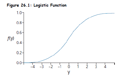
Topic 6. Logistic Function & Thresholding
-
Model Prediction:
- Set a threshold (Z)
- Estimate the probability associated with y=1
-
Specify which category observation j will belong to using the following criteria:
-
-
-
Threshold Z Selection:
- Z = 0.5 implies costs of being wrong are equal.
- If false negatives are costly (e.g., failing to detect default risk), Z can be reduced to 0.1.
-
Evaluation Metrics: For continuous variable such as rate of return, MSFE and MAFE are used.
-
MSFE (Mean Squared Forecast Error):
- MAFE (Mean Absolute Forecast Error): Similar, but uses absolute values.
-
MSFE (Mean Squared Forecast Error):
Practice Questions: Q3
Q3. For a given logistic regression model, default is assigned a value of 1 and no default is assigned a value of 0. Because the cost of default is very high on loans the bank expects its consumers to pay back, a reasonable threshold level for Z should be:
A. 0.00.
B. 0.10.
C. 0.50.
D. 0.90.
Practice Questions: Q3 Answer
Explanation: B is correct.
The Z value should be low to account for the asymmetry in risk associated with a loan that defaults (when unexpected) versus when loan payments are met (when unexpected). Setting a value equal to zero is unrealistic, and a value equal to 0.50 implies risk symmetry (which is not the case here). So, a Z of 0.10 is the most appropriate choice in this situation.
Module 2. Decision Trees, Ensemble Learning, K-Nearest Neighbors and Support Vector Machines
Topic 1. Decision Trees
Topic 2. Ensemble Learning
Topic 3. K-Nearest Neighbors (KNN)
Topic 4. Support Vector Machines (SVMs)
Topic 1. Decision Trees
- Definition: A supervised learning method that that visually represent a tree and work with sequential input features.
-
Every node of the tree has a question that reflects an observation that is connected to another node (leaf) by a branch.
-
Decision trees are useful for classification problems and continuous variable estimations and, as such, are sometimes referred to as classification and regression trees (CARTs).
-
Because CARTs are easy to interpret, they are sometimes referred to as “white-box models” as opposed to neural networks, which are considered “black-box models.”
Topic 1. Decision Trees
-
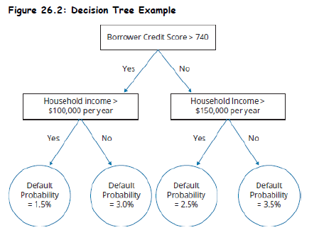
Structure:
- Root Node: Initial split based on best feature (e.g., sales increase?).
- Decision Nodes: Subsequent splits (e.g., credit sales %, earnings growth).
- Leaf Nodes (Terminal Nodes): Final classification output (e.g., default or no default).
-
Below figure shows an example of a decision tree that a bank may use to evaluate the default probability of a potential borrower.
Topic 1. Decision Trees
-
Splitting Criteria:
- Entropy:
-
Gini Index:
-
- Information Gain:
-
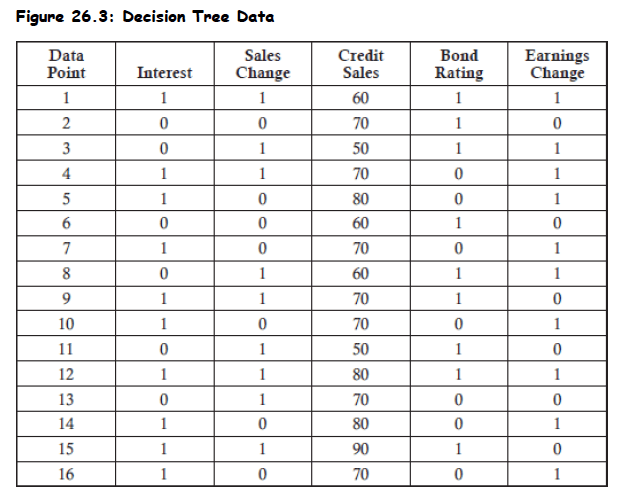
Example: Predict whether a firm will meet its interest obligations during the next fiscal year.
- Input features: sales change, bond rating, earnings change, etc.
-
Ideal Decision Tree Split:
- Perfect Split Goal: Decision tree questions should produce "pure sets" at root and decision nodes
- Pure Set: 100% of companies with earnings reductions → same outcome (did not meet obligations)
- Impure Set: 50% met obligations, 50% did not meet obligations
- Impact: Impure splits make the feature information essentially meaningless for prediction
Topic 1. Decision Trees
- Example Dataset: 16 firms analyzed for interest obligation performance - 6 firms did not meet their interest obligations and 10 firms met their interest obligations
-
The Gini coefficient for this output is computed as follows:
-
- Baseline Comparison: This number serves as the base level to compare the drop in the Gini coefficient as the tree gets larger.
- Root Node Selection: Choose variable that produces greatest decline in Gini coefficient (highest information gain)
-
-
Example: Calculation of the information gained from the sales change is shown as follows:
-
9 firms had sales increases, and 5 of those firms met interest obligations and 4 did not:
-
7 firms had sales decreases, and 5 of those firms met interest obligations and 2 did not:
-
-
-
Therefore, the information gain is equal to the base Gini measure of 0.46875 minus the weighted Gini measure of 0.45635. This results in an information gain of 0.0124.
-
9 firms had sales increases, and 5 of those firms met interest obligations and 4 did not:
- For information like the percentage of sales on credit, because it is a continuous variable that can take any value from zero to one hundred, the threshold value chosen will be the one which maximizes the information gain.
Topic 1. Decision Trees
-
The decision tree is complete when all features have been used or when a leaf is reached that is a pure set.
-
A key risk of decision trees is overfitting, which can be mitigated by setting stopping rules such that there is a maximum number of branches.
-
Overfitting Controls:
- Pre-Pruning: Stop growing tree early (e.g., if < 10 observations at a node).
- Post-Pruning: Remove branches with low predictive power after full growth.
Practice Questions: Q4
Q4. The Gini coefficient for a model is 0.375. If the weighted Gini of one of the features is 0.329, the information gain will be closest to:
A. 0.046.
B. 0.352.
C. 0.704.
D. 0.750.
Practice Questions: Q4 Answer
Explanation: A is correct.
The information gain is the difference between the base Gini and the weighted Gini. For this model, the base Gini is 0.375 and the weighted Gini is 0.329. The difference is equal to 0.375 – 0.329 = 0.046.
Topic 2. Ensemble Learning
- Ensemble of learners: Combines outputs of multiple models (often decision trees)
- 2 objectives: “Wisdom of crowds” (averaging over models) and protection against overfitting.
-
Techniques: Bootstrap Aggregation, Random Forests and Boosting
-
Bootstrap Aggregation (or Bagging): Creates multiple decision trees from training sample and aggregates their classifications/predictions
- Averaging all bagged trees reduces overall model variance compared to single tree
- Some observations may appear multiple times while others never appear in training
- “Out-of-bag” samples used to validate model.
- Pasting vs Bagging: Pasting uses sampling without replacement (e.g., 500 items → 20 sub-samples of 25 items each)
-
Random Forests: An ensemble of decision trees which is created by sampling. This process is repeated hundreds of times for a “forest” of decision trees.
-
Random forests apply bagging techniques but improve upon them by reducing the correlations between decision trees.
-
The number of features used is often equivalent to the square root of total model predictors available.
-
Model outputs with low correlations produce the greatest performance for ensembles.
-
-
Bootstrap Aggregation (or Bagging): Creates multiple decision trees from training sample and aggregates their classifications/predictions
Topic 2. Ensemble Learning
-
Boosting:
- AdaBoost: Involves a model with equal weights on all observations with sequential weight increases on misclassified outputs.
- Gradient Boosting: Fits next model to residuals of previous model.
-
Boosting consists of gradient boosting and adaptive (AdaBoost) boosting.
- Designed to improve model performance based on previously grown trees.
Practice Questions: Q5
Q5. In relation to ensembles of learners, which of the following statements best describes the “wisdom of crowds”?
A. Masses of people are never wrong.
B. It is only evident using decision trees.
C. It protects against over or underfitting.
D. It offers the benefits of averaging many predictions.
Practice Questions: Q5 Answer
Explanation: D is correct.
The wisdom of crowds is evident through ensembles of learners, where many different model predictions are made, and they can be averaged to derive a best estimate proxy. While individual models on their own are vulnerable to error, predictions from multiple models can be averaged to produce the best estimate.
Topic 3. K-Nearest Neighbors (KNN)
- Definition: A supervised machine learning model used to classify or predict the value of a target variable.
- KNN does not learn dataset relationships and is called a "lazy learner"
-
Process:
- Choose K (often √n).
- Define distance metric (e.g., Euclidean).
- Find K nearest training points.
- Assign most frequent label among neighbors.
-
Characteristics:
- No model building; makes predictions at query time.
- Works well with smaller, cleaner datasets.
-
Bias-Variance Tradeoff:
- Low K: Low bias, high variance.
- High K: High bias, low variance.
Topic 4. Support Vector Machines (SVMs)
- Definition: Supervised machine learning models, beneficial when there is a large quantity of features.
-
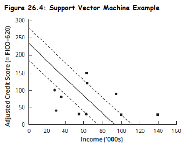
SVMs create the widest path using two parallel lines to separate the different observation classes.
-
Support vectors are the data points lying on the edge of the paths, while the separation boundary represents the center of the path.
-
Although a model with two features is the most basic, the optimization framework and underlying principles are the same regardless of how many features are modeled.
-
The output is a hyperplane with the dimension count equal to the number of features minus one.
-
Beyond a two-feature model, there will be a tradeoff between the path width and the extent of path-driven misclassifications.
-
In a simplified example where assessing borrower default incorporates only two features (e.g., credit score and income), the goal of SVMs is to use these features to develop a line that graphically separates the two groups (e.g., default versus no default).
Practice Questions: Q6
Q6. In a two-feature support vector machine, the separation boundary is best described as:
A. the center of the path.
B. the lower bound of the path.
C. the upper bound of the path.
D. all data points lying on both edges of the path.
Practice Questions: Q6 Answer
Explanation: A is correct.
In a two-feature support vector machine, the widest path using two parallel lines which separate the observations is created. Support vectors are the data points lying on the edge of the path, while the separation boundary represents the center of the path.
Module 3. Neural Networks and Model Performance
Topic 1. Neural Networks
Topic 2. Model Predictive Performance
Topic 3. ROC Curve
Topic 4. Logistic Regression vs Neural Networks
Topic 1. Neural Networks
- Concept: Artificial Neural Networks (ANNs) work in the same way as human brain
-
The feedforward network with backpropagation is the most common type of ANN.
-
Backpropagation describes how biases and weights are constantly updated through model iterations
-
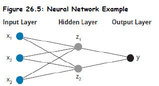
Example Architecture: 3 features (inputs), 1 single output (y) and 1 hidden layer with 2 nodes.
-
Weights (w) are applied to the inputs to determine the value of hidden layer nodes.
-
A constant bias (i.e., activation parameter) is then added, which represents how easy it is to get a node to “fire” (i.e., generate an output of 1).
-
-
- Each layer has its own activation function. A common activation function is logistic function.
-
Training: Gradient Descent algorithm is used for minimizing the objective (loss) function.
- Learning Rate: Controls step size during weight update.
-
Overfitting Risk:
- Especially with many hidden layers and nodes per layer.
- Prevented using validation sets and early stopping.
Topic 2. Model Predictive Performance
-
Evaluation Tool: For a model with binary outputs, confusion matrix can be used to evaluate model performance
- Confusion Matrix – summarizes classification results.
-
Four elements:
- True Positive (TP)
- False positive (FP)
- True Negative (TN)
- False Negative (FN)
-
Performance Metrics:
- Accuracy
- Precision
- Recall (Sensitivity)
- Error Rate
| Accuracy | Precision | Recall (Sensitivity) | Error Rate |
|---|---|---|---|
| 1- Accuracy |
Practice Questions: Q7
Q7. Which of the following statements best describes when to stop the gradient descent algorithm in a neural network model?
A. When the value for the objective function increases for both the validation set and the training set.
B. When the value for the objective function decreases for both the validation set and the training set.
C. When the value for the objective function declines for the training set, even as it improves for the validation set.
D. When the value for the objective function declines for the validation set, even as it improves for the training set.
Practice Questions: Q7 Answer
Explanation: D is correct.
To prevent overfitting, performing calculations for the validation and training datasets at the same time can be done. Moving down the valley will improve both dataset objective functions, but the point to stop the gradient descent algorithm is the point where the objective function value declines for the validation set even as it continues to improve for the training set.
Topic 3. ROC Curve
-
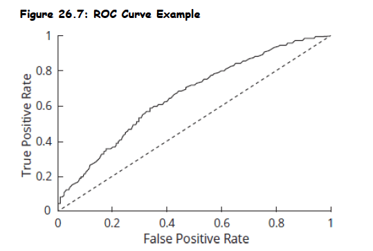
Purpose: Illustrates tradeoff between true positive rate (sensitivity) and false positive rate (1 – specificity).
- Model predictions improve as the area under the ROC curve (AUC) increases.
-
AUC (Area Under Curve):
- AUC = 1: Perfect classifier
- AUC = 0.5: No predictive value (random model)
- AUC < 0.5: Model has negative predictive value
Topic 4. Logistic Regression vs Neural Networks
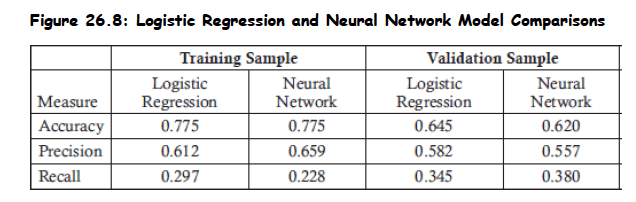
- Comparison Focus: Based on confusion matrix and metrics (accuracy, precision, recall).
- Model fit is stronger on training data as compared to validation data, implying slight overfitting.
-
Training Set:
- Both models had equal accuracy.
- Neural network had better precision.
- Logistic regression had better recall.
-
Validation Set:
- Logistic regression had higher accuracy and precision.
- Neural network had higher recall.
- Contradictory results: Use confusion matrix for better evaluation
Topic 4. Logistic Regression vs Neural Networks
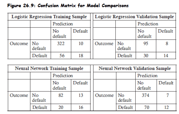
- A confusion matrix can be used to assess raw data and may better reflect the divergence.
-
One model may predict more defaults for one sample, while the other model may predict more defaults for the other sample.
-
The set with the highest true positive and true negative rates would therefore differ between the models.
Practice Questions: Q8
Q8. In a confusion matrix established for a logistic regression model, which two performance metrics must sum to 100%?
A. Precision and recall.
B. Recall and error rate.
C. Accuracy and error rate.
D. Accuracy and precision.
Practice Questions: Q8 Answer
Explanation: C is correct.
The numerator of the accuracy metric captures true positives and true negatives. The numerator of the error rate captures false positives and false negatives. Both metrics have all four outcomes in the denominator, which implies that when the metrics are added together, all four outcomes are in both the numerator and denominator. The sum must therefore be 100%.
Practice Questions: Q9
Q9. A confusion matrix on a logistic regression model shows 35 true positives, 28 false negatives, 12 false positives, and 25 true negatives. The precision metric will show a percentage output of:
A. 40%.
B. 56%.
C. 60%.
D. 74%.
Practice Questions: Q9 Answer
Explanation: D is correct.
Precision is equal to true positives (35) divided by the sum of true positives and false positives (35 + 12, or 47). 35/47 = 74%. There are 100 total outcomes (35 + 28 + 12 + 25). The error rate is the “false” outcomes (28 + 12) divided by total outcomes or 40%. Recall is the true positives (35) divided by the sum of the true positives and the false negatives (35 + 28, or 63). 35/63 = 56%. Accuracy is the “true” outcomes (35 + 25) divided by total outcomes or 60%.