Continuous measurements
of superconducting qubits:
Many-worlds to master equations

Justin Dressel
Institute for Quantum Studies, Chapman University
ICQF-2017, Patna, India, December 8 2017


Outline
-
Overview of quantum bits (qubits)
- Superconducting technology update (UC Berkeley)
-
Circuit QED modeling: resonators and transmons
-
Measuring a qubit with microwaves
- Transmission line modeling
- Many-worlds tail picture of measurement
- Stochastic quantum trajectory picture
- Dispersive coupling
-
Displacement coupling
-
Recent results
- State dragging using the quantum Zeno effect
- Measuring non-commuting observables concurrently
Abstract Quantum Bits
Quantum Bit (qubit)
- Continuum of values : Bloch sphere
- Probabilistic state:
- Evolution precesses:
- Measurement obeys Bayes' rule:
Operator Formulation:
State density operator:
Evolution precession:
Measurement update:
Superconducting Qubit: 3D Transmon
Collective motion of Cooper pairs oscillating in superconducting wires
Mesoscopic quantum coherence
Superconducting Qubit: 2D planar transmon
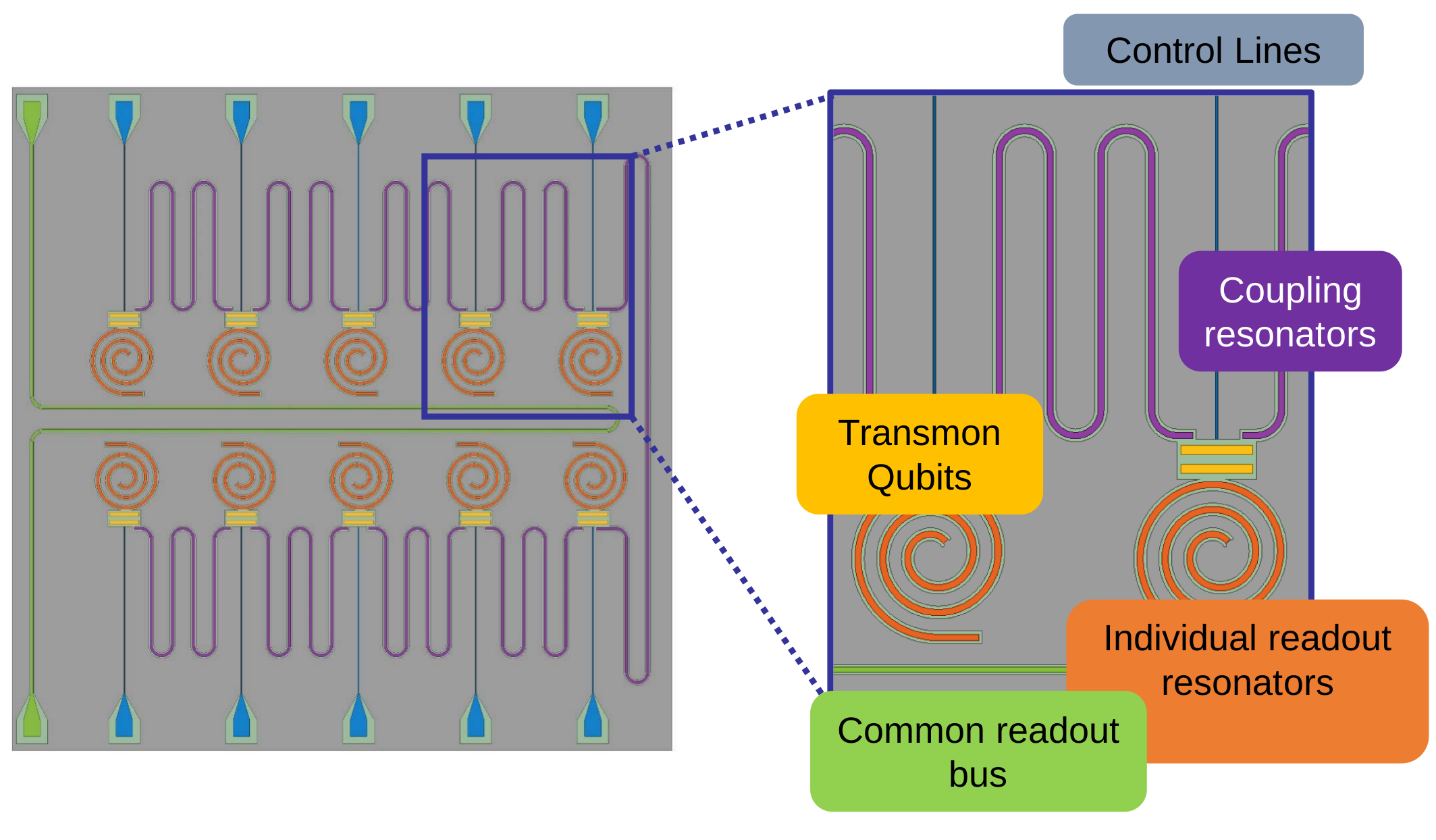
UCB 10 qubit chip design (v1)
Simultaneous 10 qubit control and readout
Python interface, Jupyter notebook display
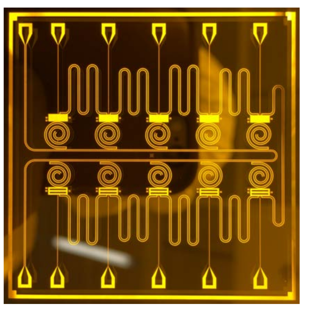
v1
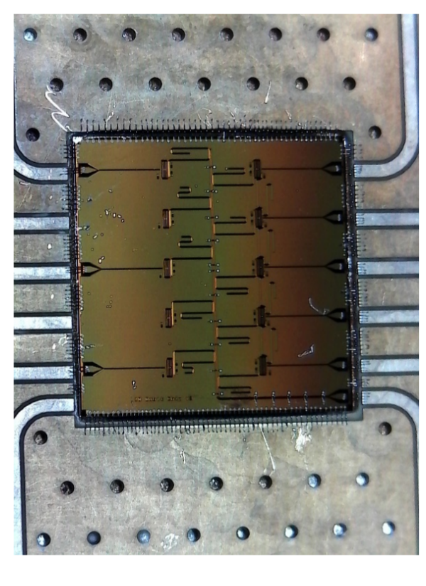
v3
Coming soon: two-layer design
separating qubits from control circuitry
Superconducting Qubit: 2D planar transmon
Circuit Quantum Electrodynamics
Ideas:
- Size scale of device (\(\mu\)m) is smaller than the characteristic wavelength of superconducting Cooper pairs: quantum coherence is relevant to the motion
- Cooper pairs (bosons) condense into collective charge motion that is well described by an effective "center of charge", much like rigid bodies are described by an effective center of mass in classical mechanics
- Collective charge motion along superconducting wires can be described by the currents and voltages it produces, which are then easily related to measurable capacitances, inductances, and impedances
- Quantization of the conjugate variables of flux and charge follows from the usual quantization of the electromagnetic field
How do we model collective mesoscopic quantum coherence?
Circuit Quantum Electrodynamics
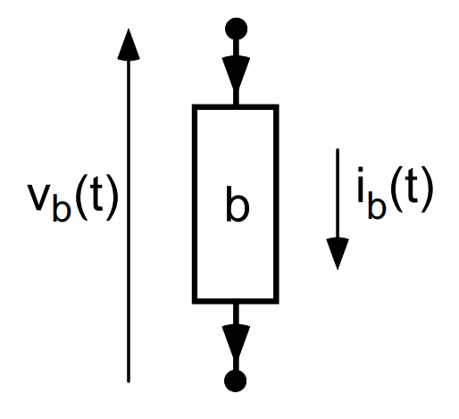
Definitions:
- Map hardware into a circuit of nodes connected by branches
Each branch is a 2-point lumped circuit element like a capacitor, inductor, etc.
- Define voltage and current for each branch via EM fields directly,
as well as the flux and charge stored in each element:
- Define reference ground node and spanning tree of active nodes connected to both capacitors and inductors - the active fluxes to ground and their time-derivatives become the key Lagrangian variables
, and (2017) . doi: 10.1002/cta.2359.
Branches \(b\in\mathcal{B}\) in spanning tree path that connects node \(n\) to ground through a sequence of capacitors
Correct conjugate charge to active node flux \(\phi_n\)
(\(+1\) capacitive, \(-1\) inductive)
Circuit Quantum Electrodynamics
- Three primary circuit elements: capacitor, inductor, and Josephson junction
Energies of node elements written in terms of canonical variables:
, and (2017) . doi: 10.1002/cta.2359.
"Kinetic" energy:
"Potential" energy:
- Quantize canonical variables for each node: (same as quantizing \(\vec{E},\vec{B}\) )
Circuit Quantum Electrodynamics
- Resonator:
, and (2017) . doi: 10.1002/cta.2359.
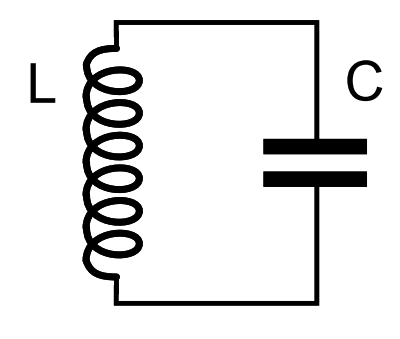
- Transmon:
Josephson junction shunted by large capacitance:
\(E_J/E_C \sim 100, \; E_J = \frac{(\hbar/2e)^2}{L_J}, \; E_C = \frac{e^2}{2C_J} \)
Circuit Quantum Electrodynamics
- Resonator + Transmon:
, and (2017) . doi: 10.1002/cta.2359.
X-X capacitive coupling
Dispersive approximation, including rotating-wave approx (RWA):
Resonator and qubit strongly detuned
Resonator frequency changes depending upon transmon energy levels
Superconducting Qubit: 3D Transmon
Qubit energy:
Superconducting Qubit: 3D Transmon
Qubit energy:
Cavity mode:
Detuned (dispersive) regime (RWA):
X-X Coupling:
Korotkov group, Phys. Rev. A 92, 012325 (2015)
Martinis group, Phys. Rev. Lett. 117, 190503 (2016)
Circuit Quantum Electrodynamics
- Resonator + Transmon + Transmission Line:
, and (2017) . doi: 10.1002/cta.2359.
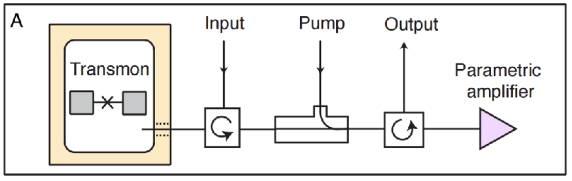
(OUT: to amplifier and detector)
(IN: from signal generator)
(2017).
Capacitance, Inductance per unit length
Circuit Quantum Electrodynamics
- Resonator + Transmon + Transmission Line:
, and (2017) . doi: 10.1002/cta.2359.
(OUT: to amplifier and detector)
(IN: from signal generator)
(2017).
Resonator decay rate near \(\omega_r\)
Boundary condition:
"Input-output relation"
Circuit Quantum Electrodynamics
- Resonator + Transmon + Transmission Line:
, and (2017) . doi: 10.1002/cta.2359.
(OUT: to amplifier and detector)
(IN: from signal generator)
(2017).
Two simplifications:
- \( \langle c_{\text{in}}(t) \rangle = -i(\varepsilon/\sqrt{\kappa}) \, e^{-i\omega_d t} \) : coherent input drive
- \(\omega_k\in[\omega_r + \frac{d\omega}{2},\omega_r - \frac{d\omega}{2}] \) : finite detector bandwidth \(d\omega\)
\( \Rightarrow dt = \frac{1}{d\omega} \) : output temporal correlation window
Many-Worlds "Tail Picture" for Evolution
- Resonator + Transmon + Transmission Line:
Koroktov, Phys. Rev. A 94, 042326 (2016)
JD group, Phys. Rev. A 96, 022311 (2017)
\(\cdots\)
- Coherent drive produces coherent resonator state, which leaks into coherent output field
- Drive + Decay = Steady state resonator field
- Per unit time \(dt\), resonator leaks amplitude \(\sqrt{\kappa dt} \) of coherent field into tail segment of width \(dx\)
- Once in tail, each \(dx\) simply propagates down the line from segment to segment
- Each segment is independent : Markov evolution
- Outgoing field and qubit state remain entangled until field is amplified and collected at the end of the transmission line
Tail stores entanglement memory of past coherent interaction of field with qubit
- Tracing out the tail produces effective "dephasing"/"decoherence" of the qubit state
- Collapsing tail pieces with measurement changes qubit amplitudes, yielding stochastic dynamics
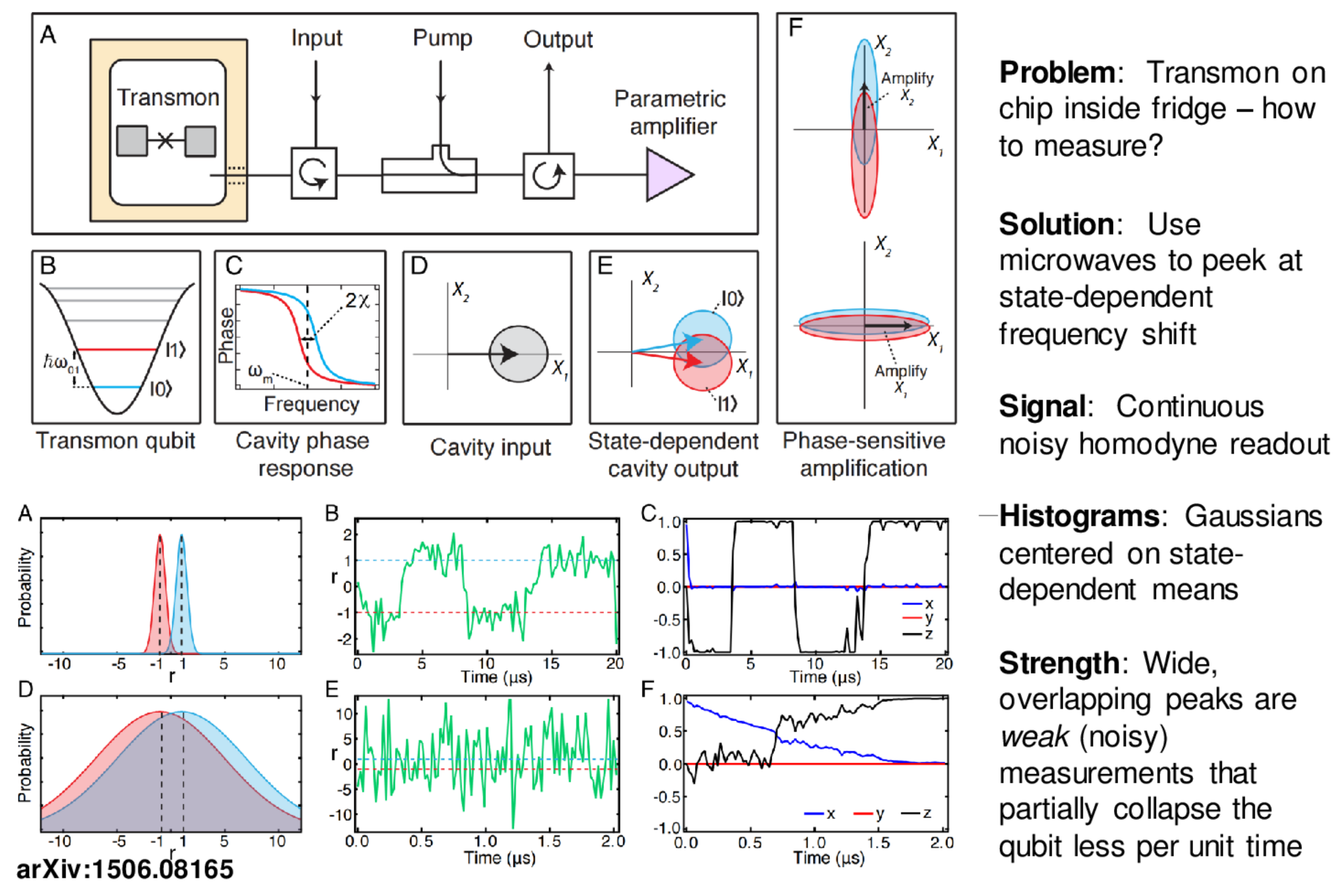
Microwave Measurement : Dispersive Coupling
Dispersive coupling:
Resonator pump:
Resonator energy decay rate:
Resonant pump produces symmetric photon number:
Only phase of resonator field is qubit-dependent
Can extract phase with homodyne measurement
Delayed Choice Dynamics!
UCB, Nature 502, 211 (2013)
Note the temporal progression:
- Field interacts with qubit in cavity
- Field leaks from cavity (unsqueezed)
- Field propagates away for a delay
- Amplifier phase chooses squeezed quadrature
- Homodyne measures squeezed quadrature
Phase of squeezing axis chosen long after field escapes cavity: type of qubit dynamics depends on this phase!
Photon Fluctuations vs. Collapse
UCB, Nature 502, 211 (2013)
Story #1:
The squeezing eliminates distinguishability of qubit states, but amplifies the intrinsic uncertainty of the cavity field photon number.
The fluctuating photon number made the qubit energy fluctuate, creating random phase drifts that dephase the qubit in the ensemble average
Story #2:
The squeezing suppresses the intrinsic photon number uncertainty, but amplifies the field separation between distinct qubit states..
The cavity photon number does not fluctuate. Instead, continuous weak monitoring of z creates partial collapses that decohere the qubit in the ensemble average
The later choice of amplification changes the physical picture,
but yields the same ensemble average.
Markovian Qubit Updates
Discrete Update Model:
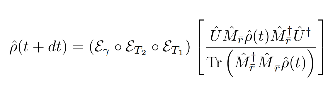
(Approximately Gaussian readout with phase-backaction, depends on quadrature phase of amplifier)
(Decomposition assumes dt much smaller than relevant evolution timescales, but longer than the relaxation timescale of resonator)
Koroktov, Phys. Rev. A 94, 042326 (2016)
JD group, Phys. Rev. A 96, 022311 (2017)
Idea:
- Measure sequence of independent amplified field segments in outgoing transmission line
- The qubit evolves naturally between measurements
These distinct evolutions compete with each other
Assumptions:
- Each measurement partially collapses the qubit state, assuming the resonator to remain in steady state
- Uncollected information leaks to environment
- The qubit energy decays on average
Phenomenological nonidealities:
(Natural qubit evolution and drive)
Stochastic master equation model:
(Ito picture - Lindblad dissipation)
(Ito picture - noise innovation)
(Ito picture - Weiner increment)
(Interpolated stochastic process)
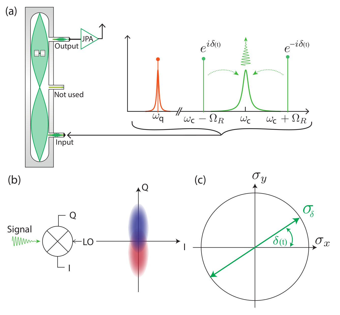
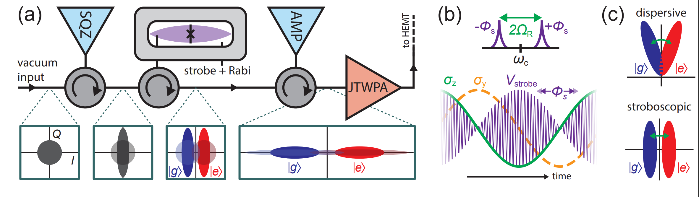
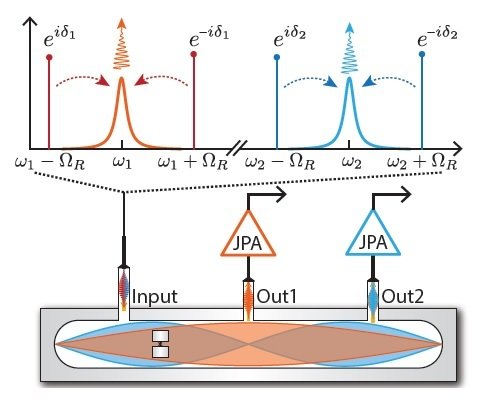
Markovian Qubit Updates: Continuous Limit
Effective causal readout:
JD group, Phys. Rev. A 94, 062119 (2016)
JD group, Phys. Rev. A 96, 022311 (2017)
- Pair of symmetrically detuned pumps
- Beats stroboscopically measure rotating qubit
- Yields displacement coupling
- Allows tunable measurement axis
- Multiple cavity modes = multiple observables
- Allows squeezed pump field (arXiv:1708.01674)
Displacement coupling:
Siddiqi group, Nature 538, 491 (2016)
Microwave Measurement : Displacement Coupling
Rotating frame:
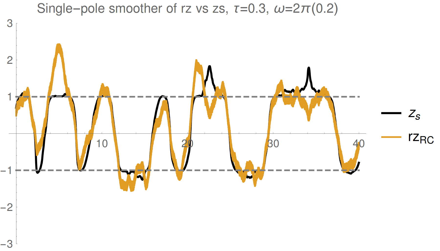
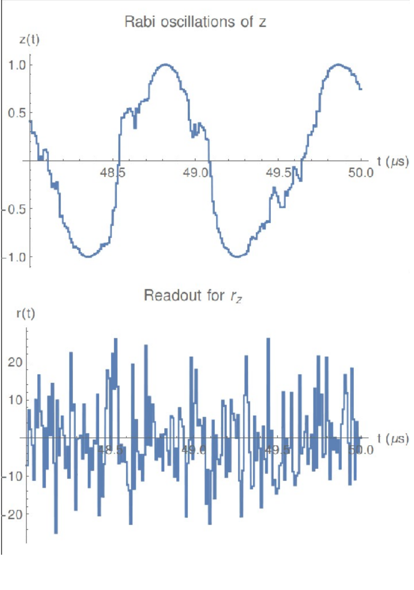
Result: Incoherent Qubit Gate using Quantum Zeno Effect
Idea : use time-varying measurement axes to drag the quantum state around the Bloch sphere using the quantum Zeno effect
The record tracks the state well in this regime, so can be used as a herald for high-fidelity gates
Non-unitary gate
(measurement-based)
Stroboscopic displacement coupling can have time-varying side-lobe phases
JD, Siddiqi group, arXiv:1706.08577
Jumps : Faster drag speeds allow trajectories to jump to the opposite pole, decreasing ensemble-averaged dragging fidelity
Jump-axis : Dragging dynamics causes lag of actual Zeno-pinned behind the measurement axis by a fixed angle
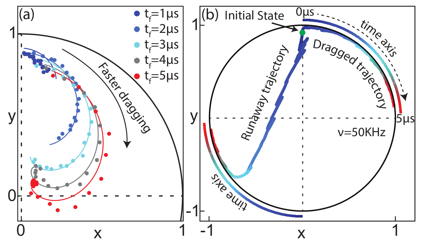
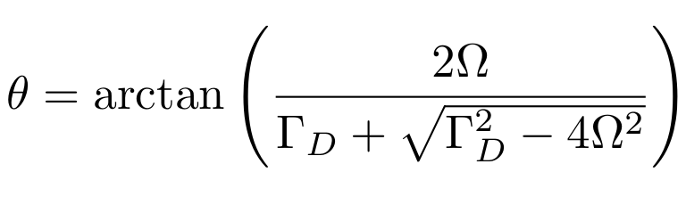
JD, Siddiqi group, arXiv:1706.08577
Pinned to poles : Other than the jumps, state remain pinned to lagged measurement poles
Result: Incoherent Qubit Gate using Quantum Zeno Effect
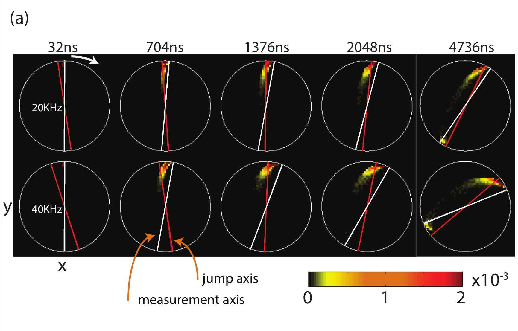
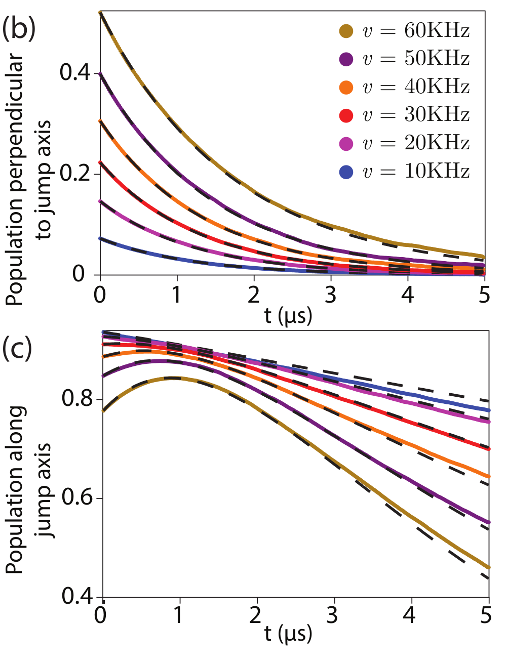
State collapses to jump-axis
JD, Siddiqi group, arXiv:1706.08577
Result: Incoherent Qubit Gate using Quantum Zeno Effect
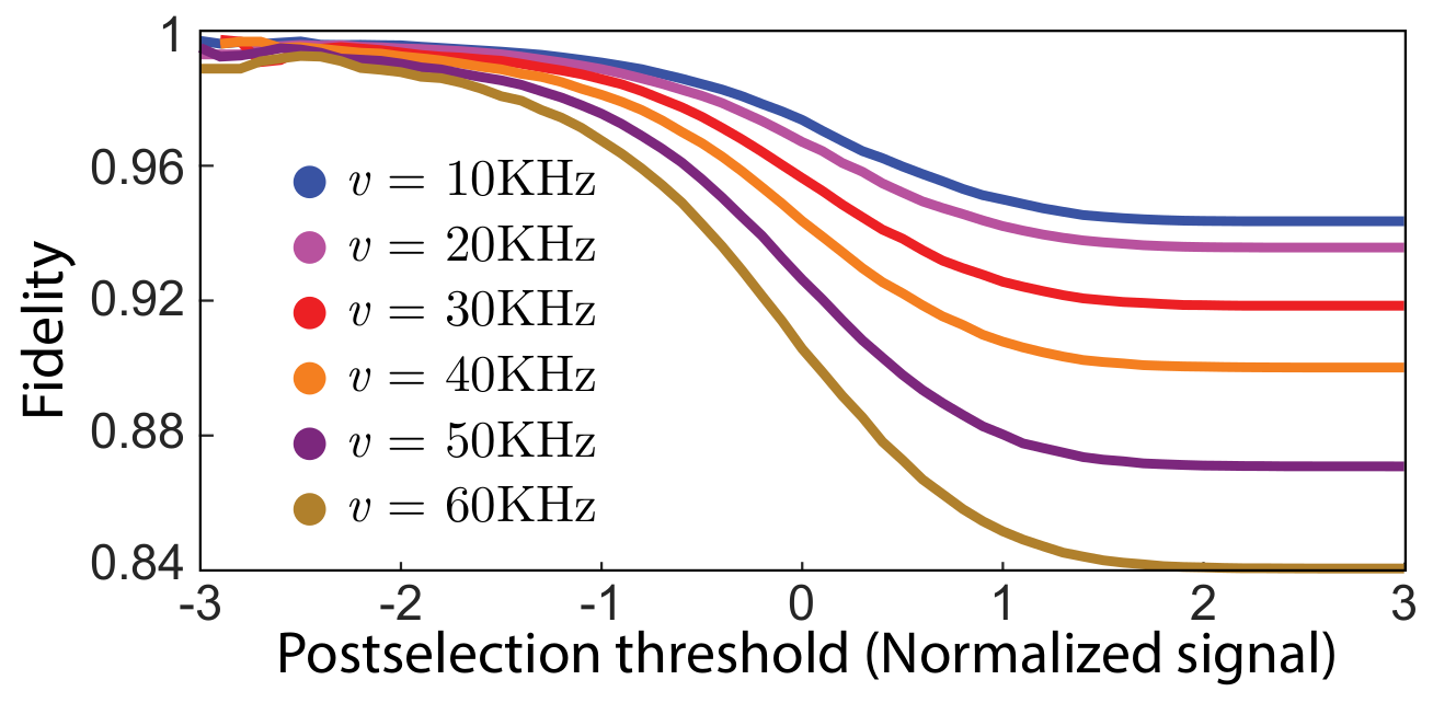
Post-selecting on trajectories with an average readout with a value >1 keeps only trajectories that did not jump, heralding a reasonably high-fidelity dragging gate for that subset
Alternatively, the jump may be observed, then corrected later
Result: Incoherent Qubit Gate using Quantum Zeno Effect
Siddiqi group, Nature 538, 491 (2016)
4 pumps, symmetrically detuned from
2 resonator modes of 3D transmon
2 simultaneous noncommuting observables
Result : Simultaneous Noncommuting Observable Measurement
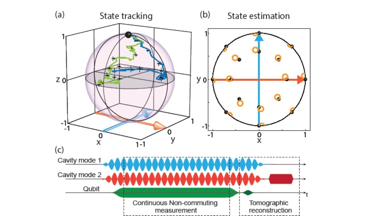
Siddiqi group, Nature 538, 491 (2016)
Observable incompatibility leads to diffusion around Bloch sphere
Result : Simultaneous Noncommuting Observable Measurement
Basins of attraction if measurement axes are nearly aligned
Siddiqi group, Nature 538, 491 (2016)
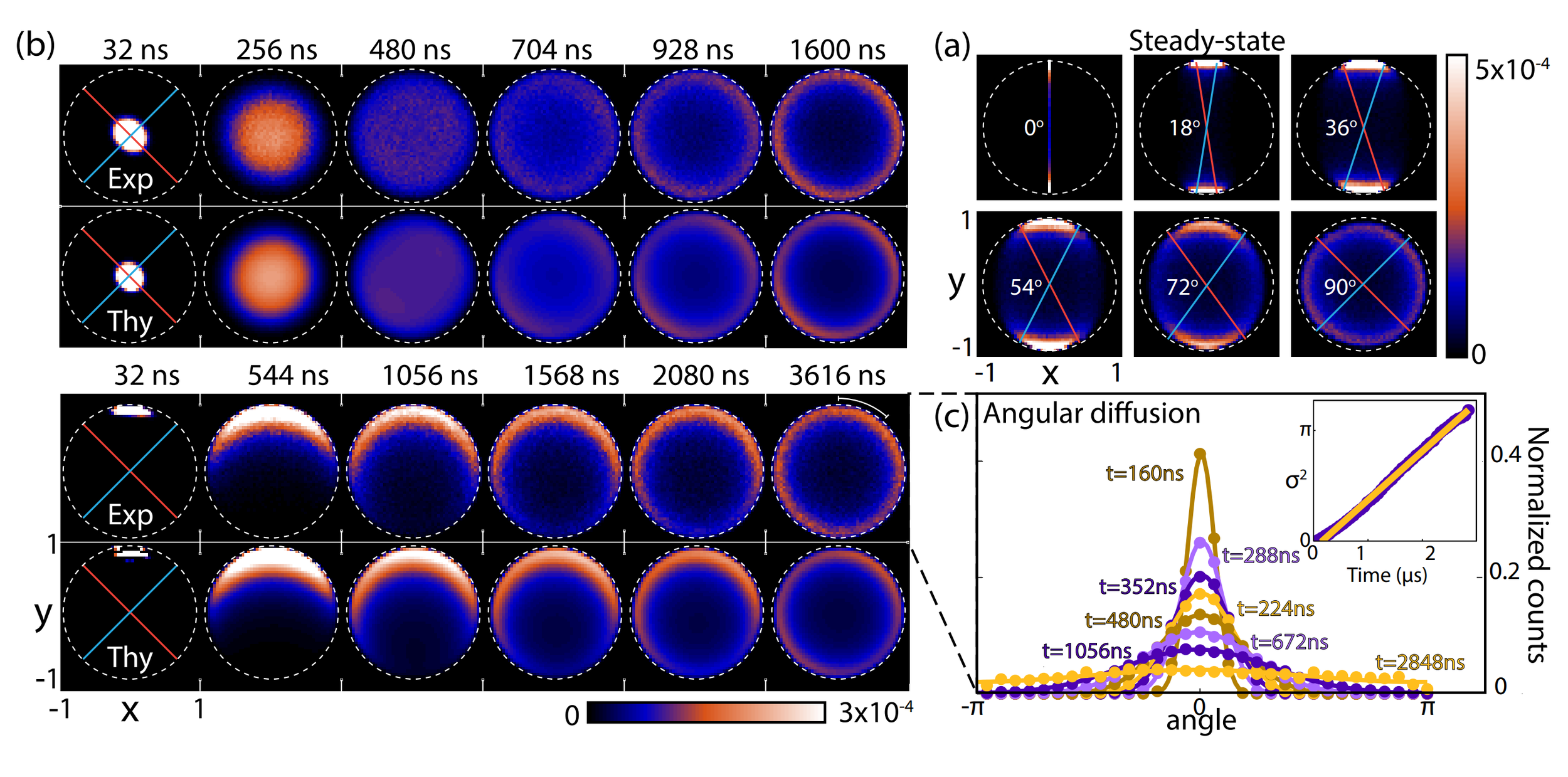
Result : Simultaneous Noncommuting Observable Measurement
State disturbance can be measured
Result agrees with the lower bound set by the Maccone-Pati relation involving the sum of variances:
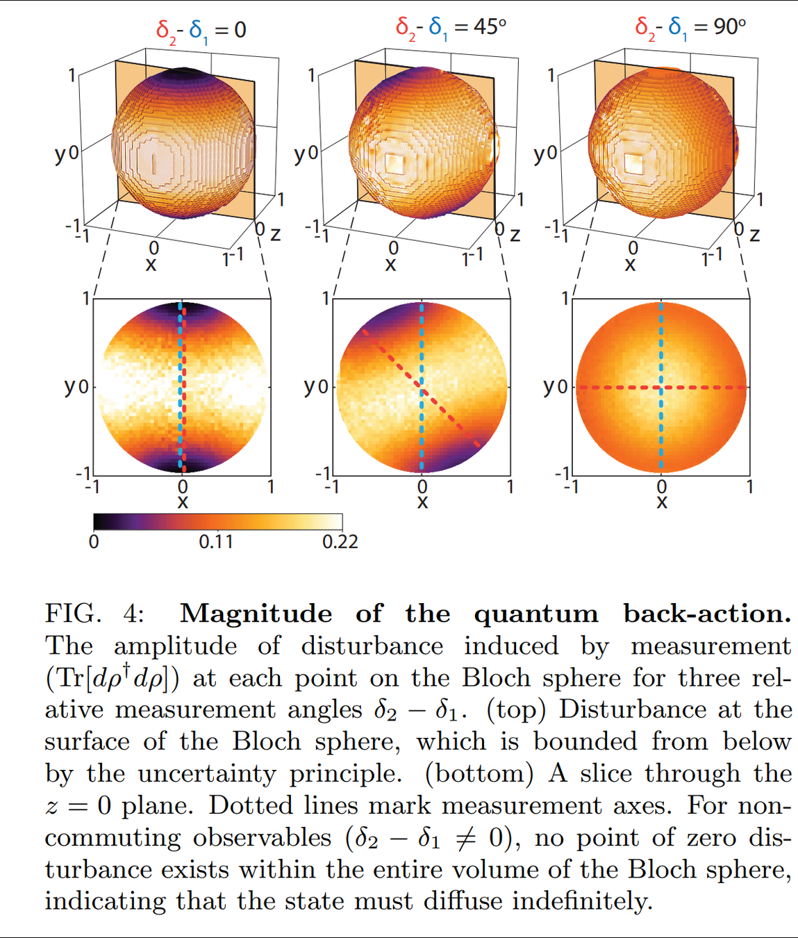
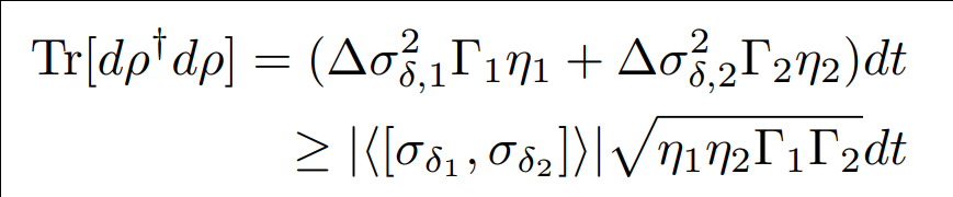
Uncertainty relation forces the random state diffusion when measuring incompatible axes
Conclusions
- Continuous measurements and quantum trajectories can now be used in the laboratory with superconducting transmon circuits
- 10+ qubit planar 2D transmon designs in-hand at UCB
- Both dispersive and displacement measurements are possible
- Dynamics can be modeled unitarily (many-worlds) or stochastically (simpler)
- The quantum Zeno effect can produce a measurement-based gate by dragging the state along with a time-dependent axis
- Multiple noncommuting observables can be measured simultaneously
- Lots more, and more to come
Thank you!