Strengthening weak measurements for qubit multitime correlators

Justin Dressel
Razieh Mohseninia, Jose Raul Gonzalez Alonso
Mordecai Waegell, Nicole Yunger Halpern
PIMan Workshop 2019
Chapman University
March 20, 2019

An Unexpected Question

https://quantumfrontiers.com/2018/09/23/doctrine-of-the-measurement-mean/
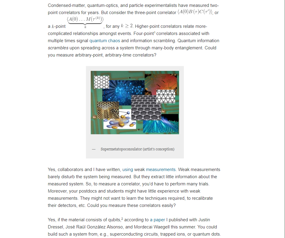
"Four-point [out-of-time-ordered] correlators ... signal quantum chaos and information scrambling." Can we measure them?"
Nicole Yunger Halpern
What is an Out-of-Time-Ordered Correlator (OTOC)?
(and why should I care?)
Idea (Kitaev) :
- Poisson brackets of canonically conjugated variables at different times signal classical chaos as Lyapunov exponential divergence
- Promoting brackets to quantum case suggests we examine the (average of the square of) the commutator instead to isolate such behavior
- For commutators of unitary operators, an OTOC is the only nontrivial quantity that remains
- Since persistent information scrambling is a hallmark of classical chaos, we guess that the OTOC witnesses quantum information scrambling
Noncommutativity causes decay
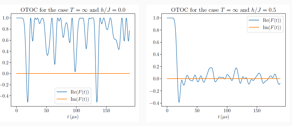
Non-integrable spin chain example
Integrable
Non-Integrable
V and W of OTOC are spin Z operators at opposite ends of a 5-spin chain
persistent decay
But is such an OTOC measurable in the lab?
(after all, it's non-Hermitian)
Initial Answer :
- This looks suspiciously similar to the non-Hermitian structure of the Kirkwood-Dirac (KD) quasiprobability distribution
- KD is closely related to the quantum weak value, and can be determined from weak measurements
- The OTOC is similarly measurable using weak measurement sequences, and is determined by an extended KD quasiprobability distribution
OTOC:
(probability of b)
(quantum weak value)
(KD distribution)
Yunger Halpern, Swingle, JD PRA 9, 042105 (2018)

Non-integrable spin chain: OTOC revisited
Blue : Ideal Orange : Weak Measurement
With finite temperature and decoherence added, OTOC as witness is less convincing
Gonzalez Alonso, JD et al. PRL 122, 040404 (2019)
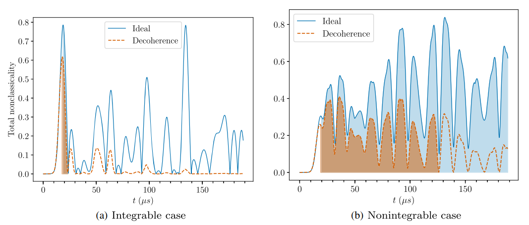
Non-integrable spin chain: OTOC KD QPD
Timescales in OTOC extended KD QPD Nonclassicality still clearly distinguish two dynamical cases
Gonzalez Alonso, JD et al. PRL 122, 040404 (2019)
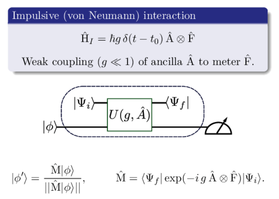
Recall (Weak) Indirect Measurement
Measurement produces a channel-valued measure (instrument), not just POVM
This procedure can be repeated many times in a row
Easy circuit : prepare ancilla, entangling gate, measure ancilla
Pang, Dressel, Brun, PRL 113, 030401 (2014)
The most interesting measurement in the world
Crude idea : measurement operator approximately linearizes in weak measurement regime (linear response regime)
Post-interaction system state couples to anticommutator to linear order in coupling:
Sequences of measurements create nested anticommutator terms to lowest order in the joint couplings
Anticommutator for measurement
"Non-Hermitian" term:
real part of KD distribution
Background terms, can be subtracted away once measured independently
"small"
Note: unitary transformation yields commutator instead
-
Benefit : Isolating such a nested commutator term in measurement sequence gives access to interesting non-Hermitian terms like those that appear in OTOCs and the weak value
-
Annoyance : Isolating this term means subtracting away unwanted terms, including the calibrated background and any higher-order terms, which is difficult in practice
- Miracle : For qubits, the anticommutator terms can be isolated exactly using any measurement strengths g
JD, et al. PRA 98, 012032 (2018)

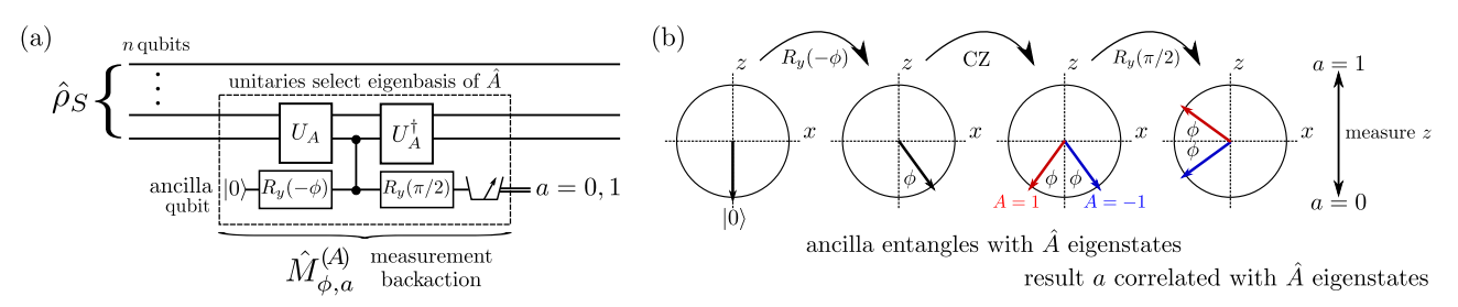
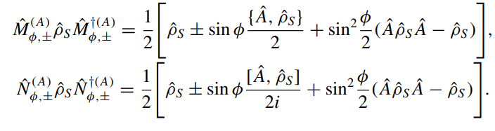
Arbitrary Strength Qubit Measurements
Informative Measurement:
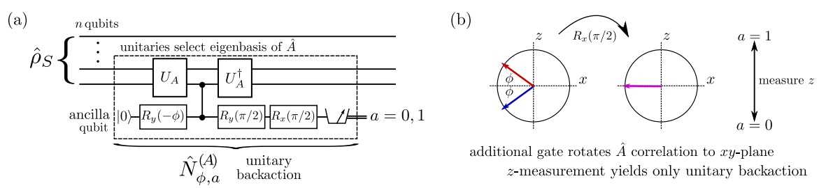
Non-Informative Measurement:
JD, et al. PRA 98, 012032 (2018)
Generalized spectral decomposition
(Works for observables A that square to the identity)
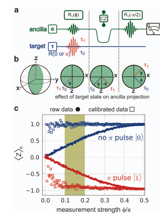
Tested in the Laboratory!
Informative Measurement:
White, Mutus, JD, et al. npj Quantum Information 2, 15022 (2016)
Generalized spectral decomposition
"rescales response curves"
Generalized measurement method used experimentally with superconducting qubits (Google)
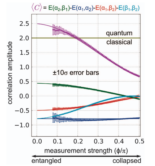
Bell-Leggett-Garg Inequality violation with weak measurements
Informative Measurement:
White, Mutus, JD, et al. npj Quantum Information 2, 15022 (2016)
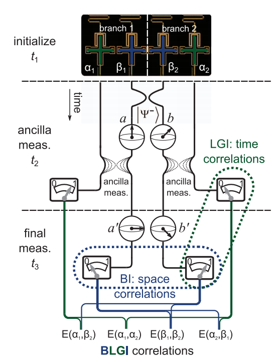
- Avoids "clumsiness loophole" by only correlating nonlocal measurements
- Avoids "fair sampling" loophole by using one experimental ensemble
- Requires weak measurements to see violation (preserve entanglement)
Informative Qubit Measurements
JD, et al. PRA 98, 012032 (2018)
Useful corollaries:
Anticommutators isolated perfectly for any coupling strength
Nested anticommutator averages can be measured directly for any coupling strength
Non-Informative Qubit Measurements
JD, et al. PRA 98, 012032 (2018)
Useful corollaries:
Commutators also isolated perfectly for any coupling strength
Nested commutator averages can also be measured directly for any coupling strength
Any strength? What happened to state collapse?
JD, et al. PRA 98, 012032 (2018)
Why does this work? Examine full transformation:
(Lindblad) decoherence terms from the measurement cancel in Pauli-like averages
However, marginalization of results will reveal the collapse-based disturbance
Application: Strongly Measured 2-Point Correlator
JD, et al. PRA 98, 012032 (2018)
2-point temporal qubit correlators may be indirectly measured using any coupling strength
These are common theoretical objects that are usually considered inaccessible to measurement
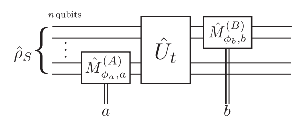
Bracketing measurement by unitary evolutions probes a Heisenberg-evolved operator
The final unitary may be omitted as inconsequential to the measured average
Application: Strongly Measured 4-Point Correlator
JD, et al. PRA 98, 012032 (2018)
4-point temporal qubit out-of-time-ordered correlators may be directly measured using any measurement strength
This directly recovers the desired OTOC and squared commutator connected with information scrambling and chaos
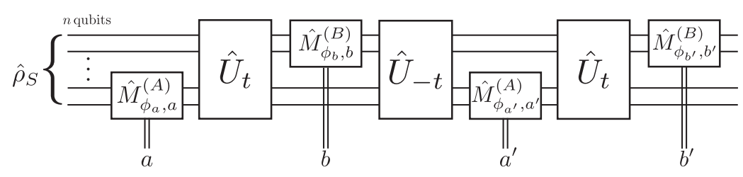
(one reversed evolution needed)
Conclusions
- Out-of-time-ordered correlators roughly witness information scrambling
- Nested (anti)commutators are measurable for qubits with any strength
- 2- and 4-point qubit correlators can be directly measured
- Follow-up research in preparation:
- Measuring qubit quasiprobabilities strongly with several techniques
- Measuring qutrit correlators with arbitrary strength
- Investigation of out-of-time-ordered correlators experimentally
Thank you!
Superconducting Qubits
Mesoscopic quantum coherence of collective charge motion at \(\mu\)m scale
EM Fields produced by charge motion described by Circuit QED
Lowest levels of anharmonic oscillator potentials treated as artificial atoms
Typical Transmon Parameters
"3D Transmon"
Cavity mode:
Detuned (dispersive) regime (RWA):
X-X Coupling:
Korotkov group, Phys. Rev. A 92, 012325 (2015)
Martinis group, Phys. Rev. Lett. 117, 190503 (2016)
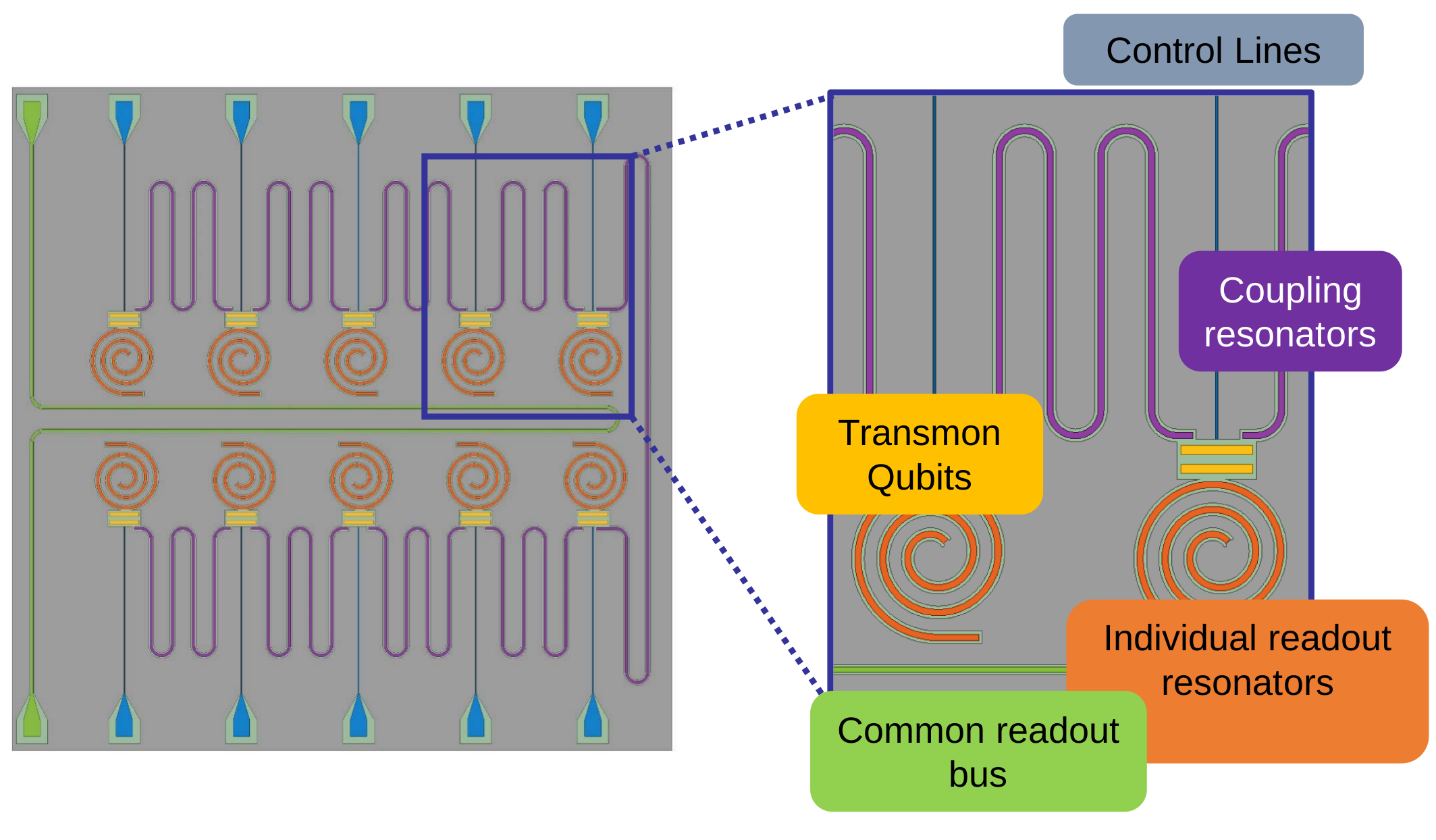
2D planar chip schematic
Bus acts as Purcell filter, coupled to traveling wave parametric amplifier (TWPA)
Similar parameters:
v1
v3
Coming soon: two-layer design of 20+ qubits
separated from control circuitry
(similar to Google Bristlecone + IBM Q)
Now on v8+
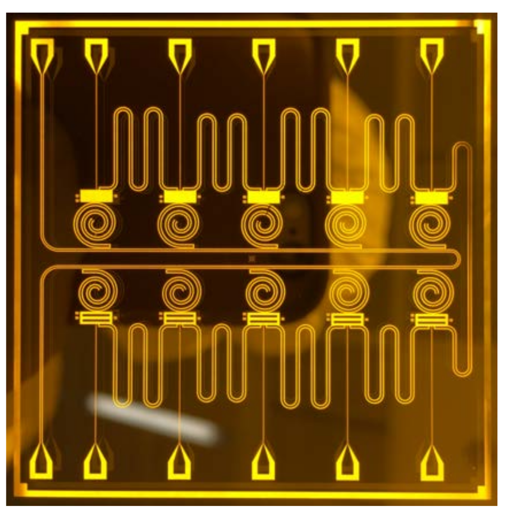
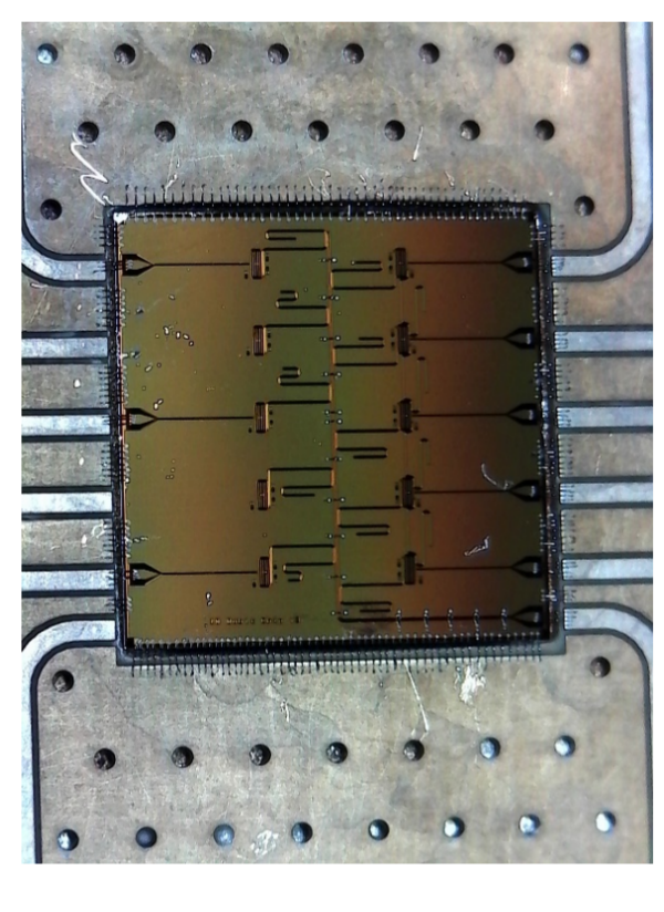
UCB 2D planar chip
Multiplexed 10 qubit control and readout
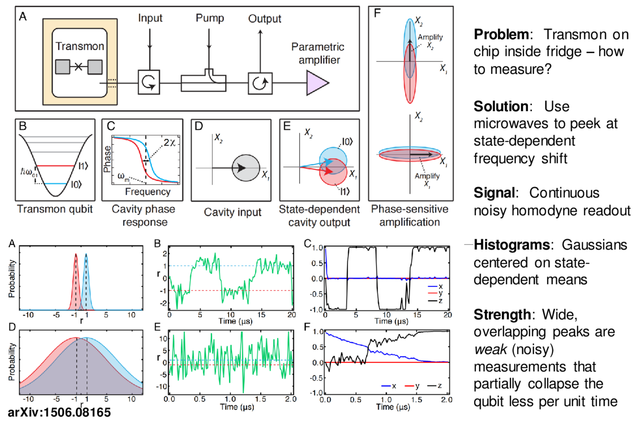
Single shot "projective" readout :
typical quantum computing goal