Watching a quantum system:
How to continuously measure a superconducting qubit


Justin Dressel
Institute for Quantum Studies, Chapman University
University of Wisconsin, Madison, October 26th 2017




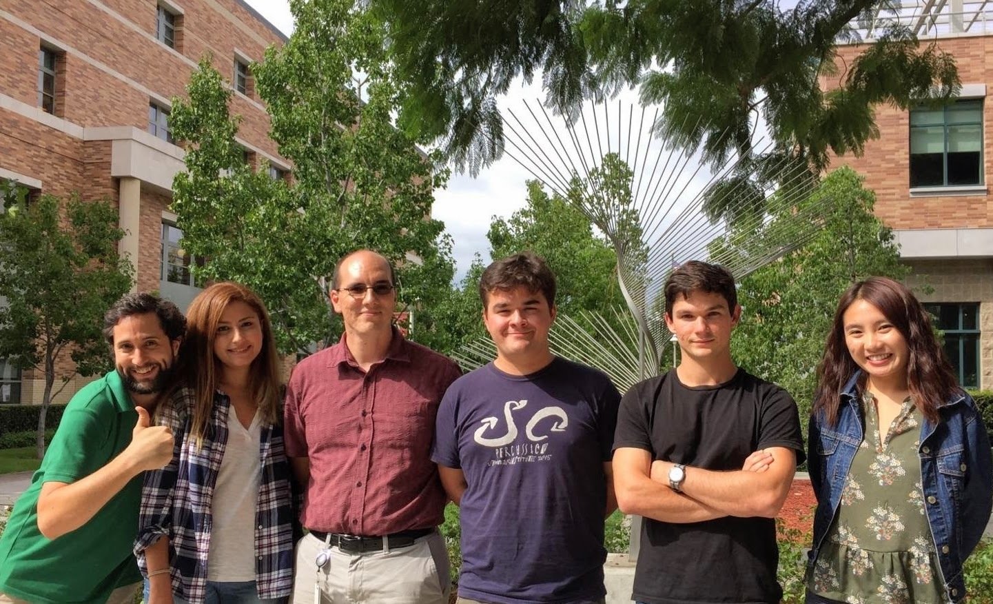
Current Group
Justin Dressel
José Raúl Gonzales Alonso (postdoc)
Shiva Lotfallahzadeh Barzili (grad student)
Aaron Grisez (undergrad)
Amy Lam (undergrad)
Michael Seaman (undergrad)
William Parker (undergrad)
Luis Pedro García-Pintos (postdoc - now at UMB)
Taylor Lee Patti (undergrad - now at Harvard)


Outline
-
Overview of quantum bits (qubits)
-
Superconducting technology update (UC Berkeley)
-
Superconducting technology update (UC Berkeley)
-
Measuring a qubit with microwaves
- Dispersive coupling
-
Displacement coupling
-
Recent results
- State dragging using the quantum Zeno effect
- Measuring non-commuting observables concurrently
- State tomography via classical signal filtering
- Smoothed past observable estimates and readout
Overview of Quantum Bits
Classical Bit
- 2 values : 0 or 1
- Probabilistic state:
- Evolution can only flip:
- Measurement obeys Bayes' rule:
Quantum Bit (qubit)
- Continuum of values : Bloch sphere
- Probabilistic state:
- Evolution precesses:
- Measurement obeys Bayes' rule:
Overview of Quantum Bits
Quantum Bit (qubit)
- Continuum of values : Bloch sphere
- Probabilistic state:
- Evolution precesses:
- Measurement obeys Bayes' rule:
Operator Formulation:
State density operator:
Evolution precession:
Measurement update:
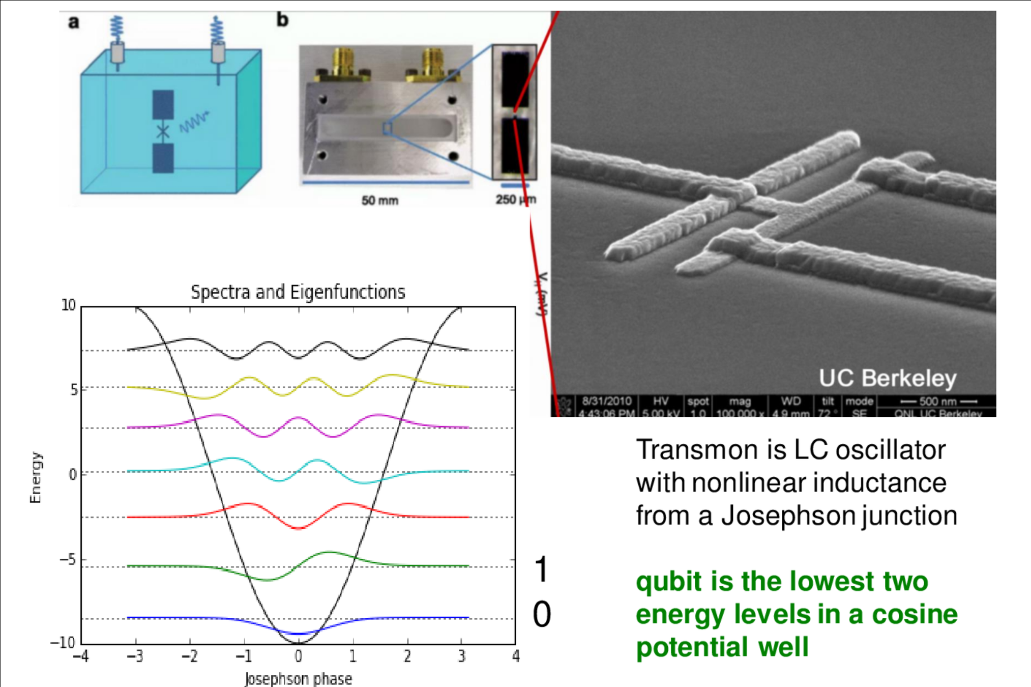
Superconducting Qubit: 3D Transmon
Qubit energy:

Superconducting Qubit: 3D Transmon
Qubit energy:
Cavity mode:
Detuned (dispersive) regime (RWA):
X-X Coupling:
Korotkov group, Phys. Rev. A 92, 012325 (2015)
Martinis group, Phys. Rev. Lett. 117, 190503 (2016)
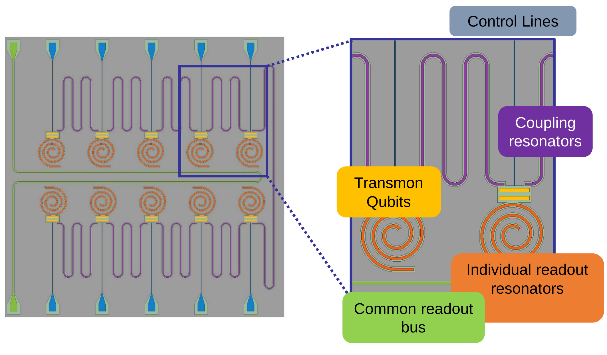
Superconducting Qubit: 2D planar transmon

UCB 10 qubit chip design (v1)
Simultaneous 10 qubit control and readout
Python interface, Jupyter notebook display
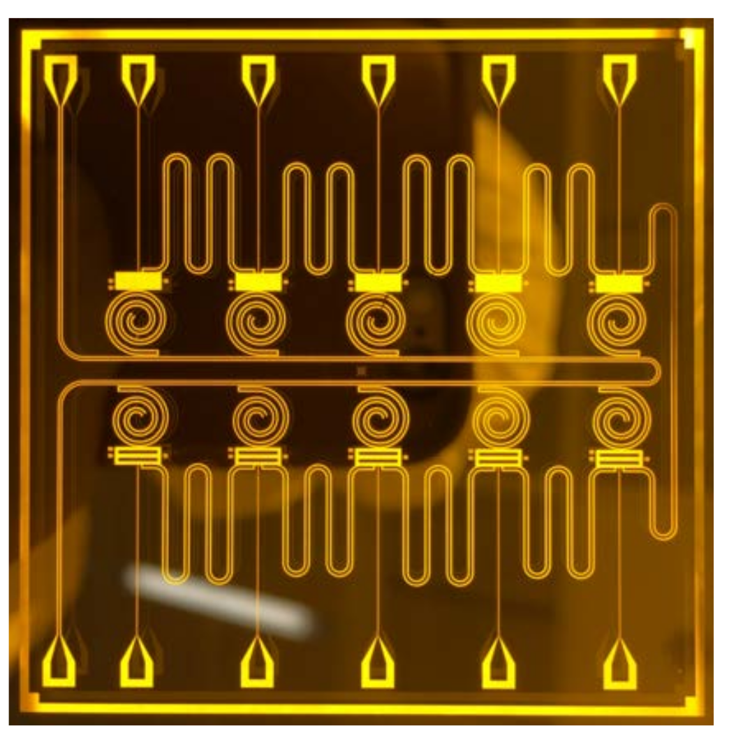
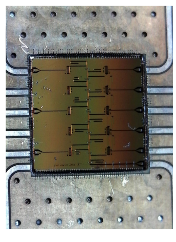
v1
v3
Coming soon: two-layer design
separating qubits from control circuitry
Superconducting Qubit: 2D planar transmon
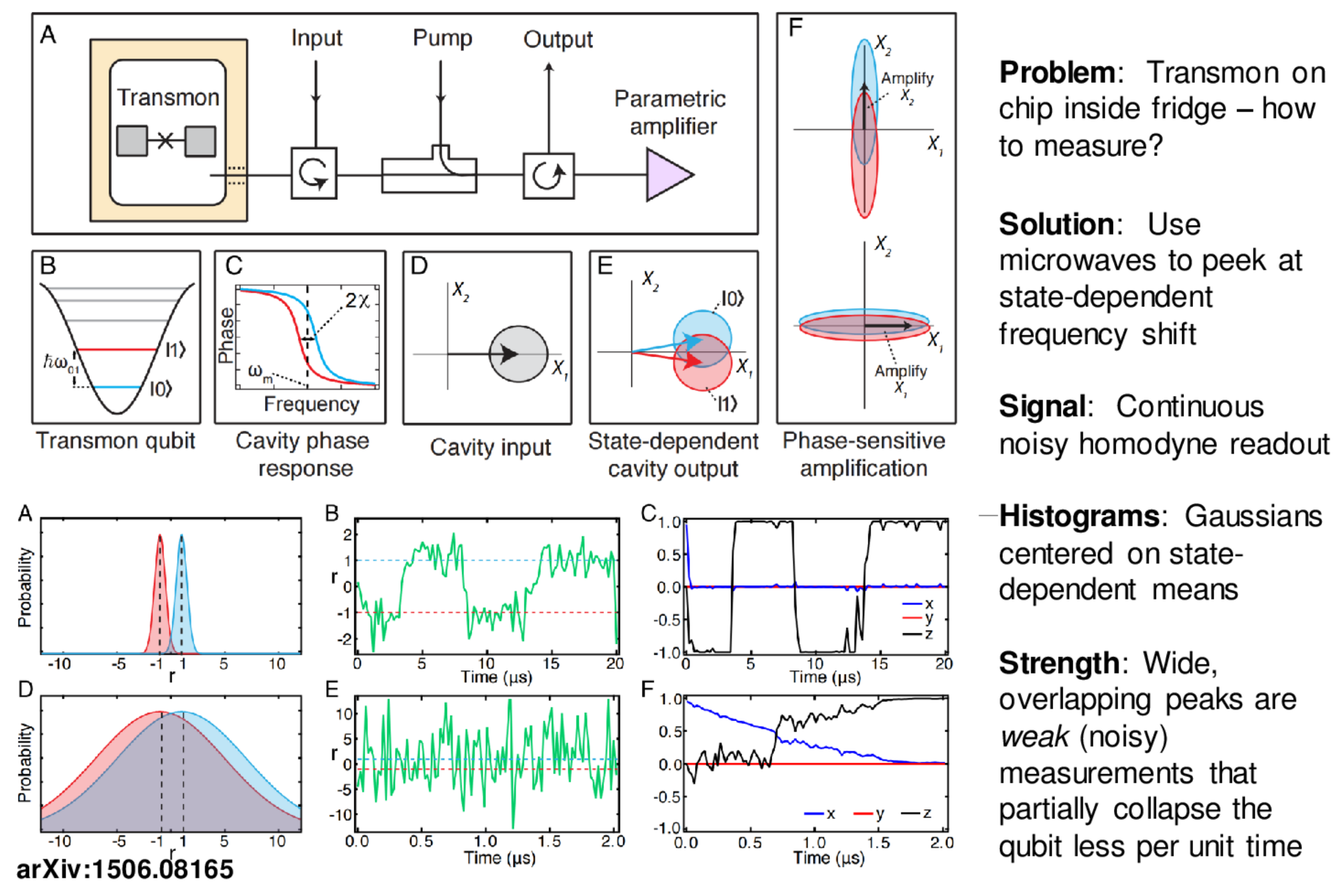
Microwave Measurement : Dispersive Coupling
Dispersive coupling:
Resonator pump:
Resonator energy decay rate:
Resonant pump produces symmetric photon number:
Only phase of resonator field is qubit-dependent
Can extract phase with homodyne measurement
Markovian Qubit Updates
Discrete Update Model:
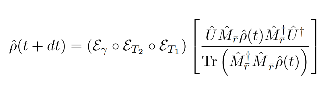
(Approximately Gaussian readout with phase-backaction, depends on quadrature phase of amplifier)
(Decomposition assumes dt much smaller than relevant evolution timescales, but longer than the relaxation timescale of resonator)
Koroktov, Phys. Rev. A 94, 042326 (2016)
JD group, Phys. Rev. A 96, 022311 (2017)
Idea:
- Measure sequence of independent amplified field segments in outgoing transmission line
- The qubit evolves naturally between measurements
These distinct evolutions compete with each other
Assumptions:
- Each measurement partially collapses the qubit state, assuming the resonator to remain in steady state
- Uncollected information leaks to environment
- The qubit energy decays on average
Phenomenological nonidealities:
(Natural qubit evolution and drive)
Stochastic master equation model:
(Ito picture - Lindblad dissipation)
(Ito picture - noise innovation)
(Ito picture - Weiner increment)
(Interpolated stochastic process)
Markovian Qubit Updates: Continuous Limit
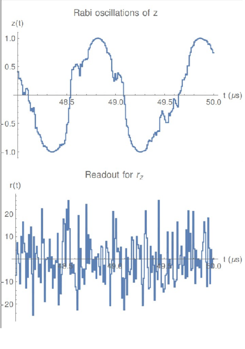
Effective causal readout:
Note: Follows expectation value of Z. We will return to this.
JD group, Phys. Rev. A 94, 062119 (2016)
JD group, Phys. Rev. A 96, 022311 (2017)
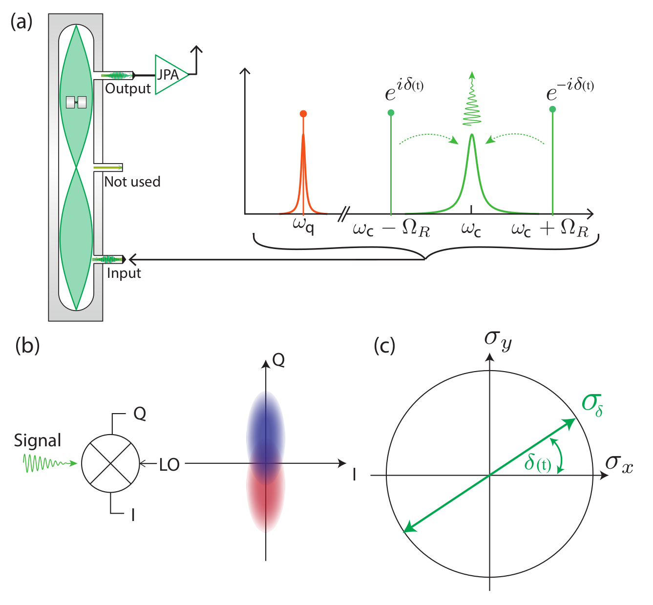
- Pair of symmetrically detuned pumps
- Beats stroboscopically measure rotating qubit
- Yields displacement coupling
- Allows tunable measurement axis
- Multiple cavity modes = multiple observables
- Allows squeezed pump field (arXiv:1708.01674)
Displacement coupling:
Siddiqi group, Nature 538, 491 (2016)
Microwave Measurement : Displacement Coupling
Rotating frame:

Result: Incoherent Qubit Gate using Quantum Zeno Effect
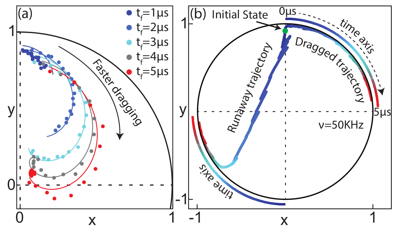
Idea : use time-varying measurement axes to drag the quantum state around the Bloch sphere using the quantum Zeno effect
The record tracks the state well in this regime, so can be used as a herald for high-fidelity gates
Non-unitary gate
(measurement-based)

Stroboscopic displacement coupling can have time-varying side-lobe phases
JD, Siddiqi group, arXiv:1706.08577
Jumps : Faster drag speeds allow trajectories to jump to the opposite pole, decreasing ensemble-averaged dragging fidelity
Jump-axis : Dragging dynamics causes lag of actual Zeno-pinned behind the measurement axis by a fixed angle


JD, Siddiqi group, arXiv:1706.08577
Pinned to poles : Other than the jumps, state remain pinned to lagged measurement poles
Result: Incoherent Qubit Gate using Quantum Zeno Effect
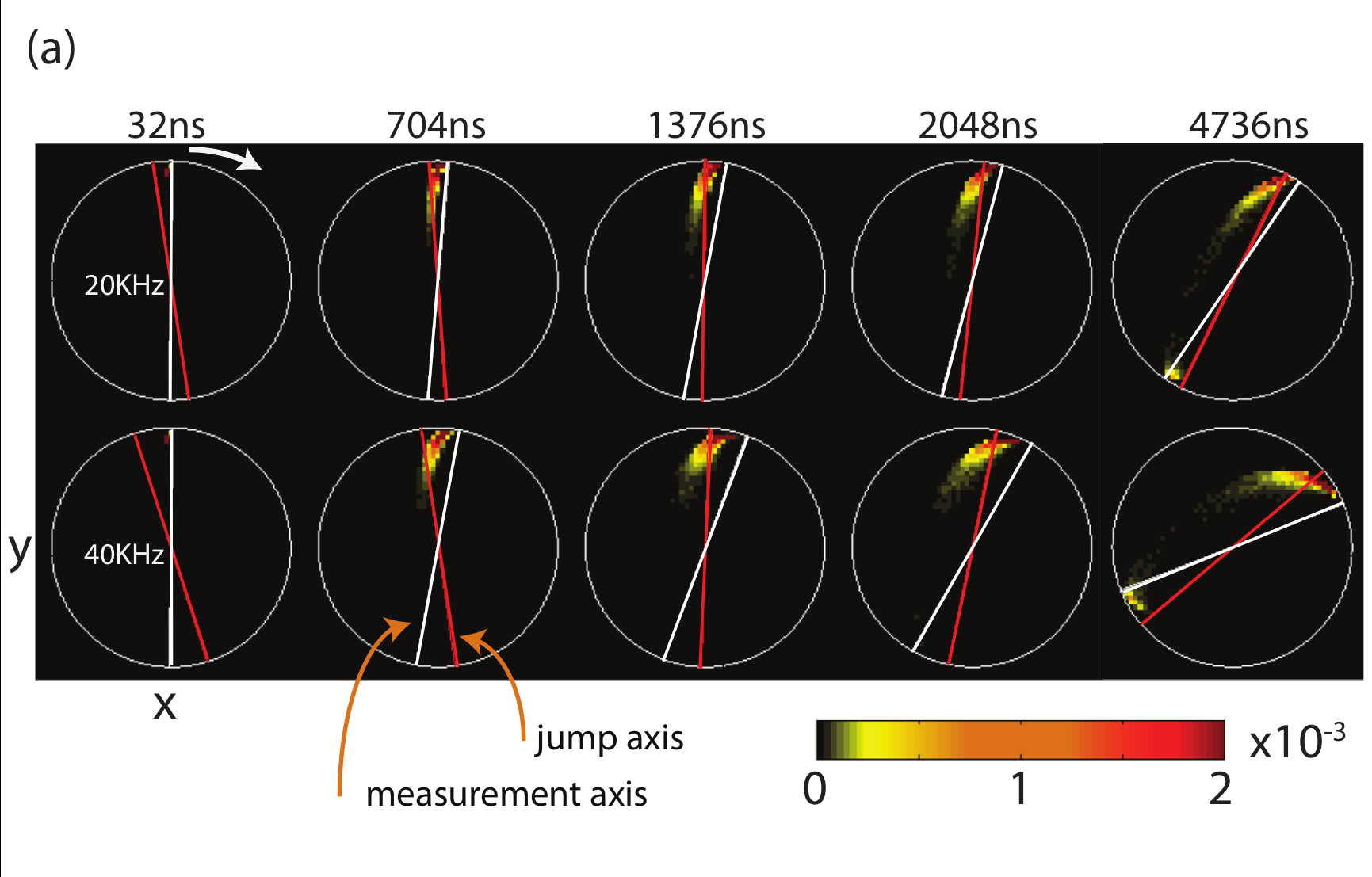

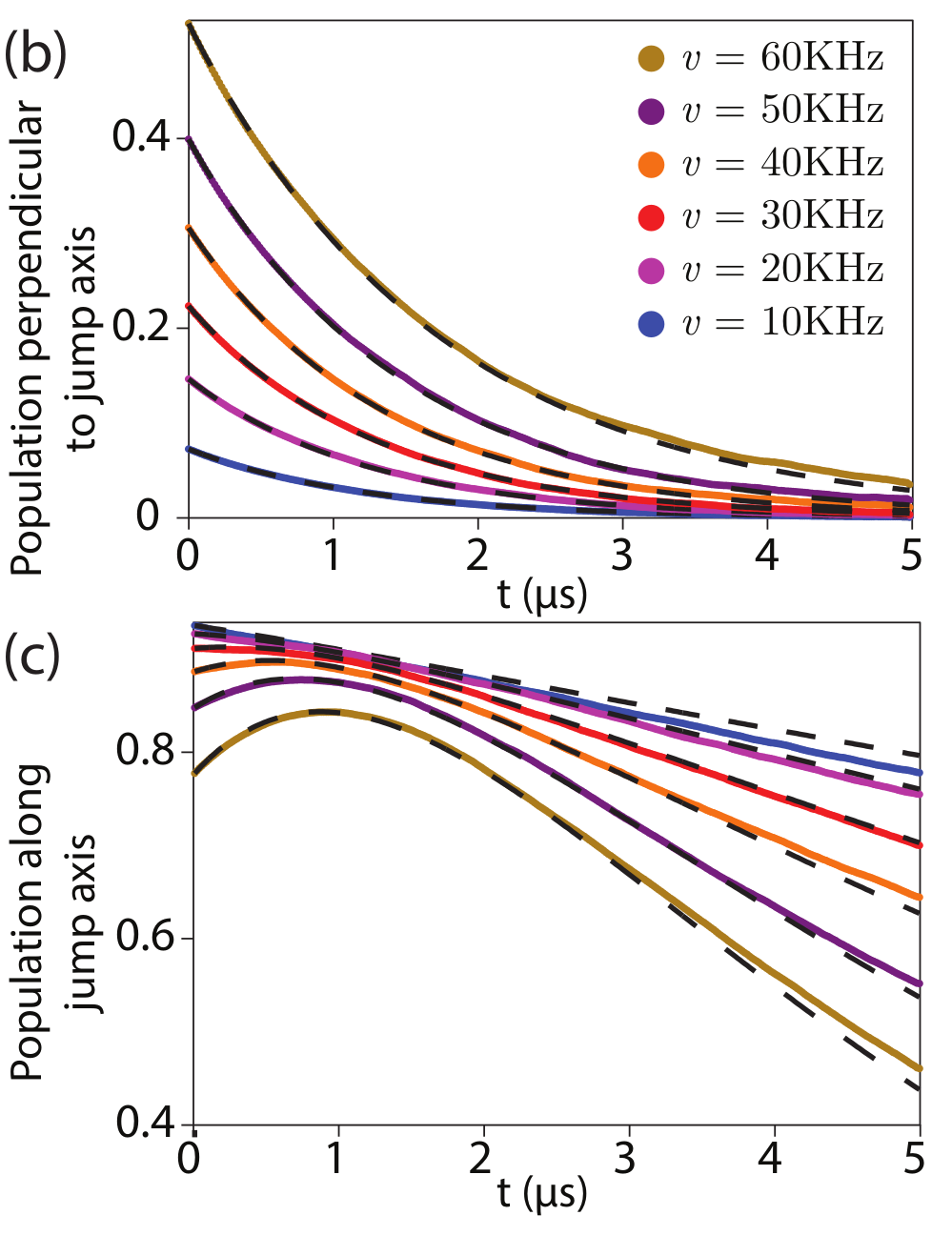
State collapses to jump-axis
JD, Siddiqi group, arXiv:1706.08577
Result: Incoherent Qubit Gate using Quantum Zeno Effect

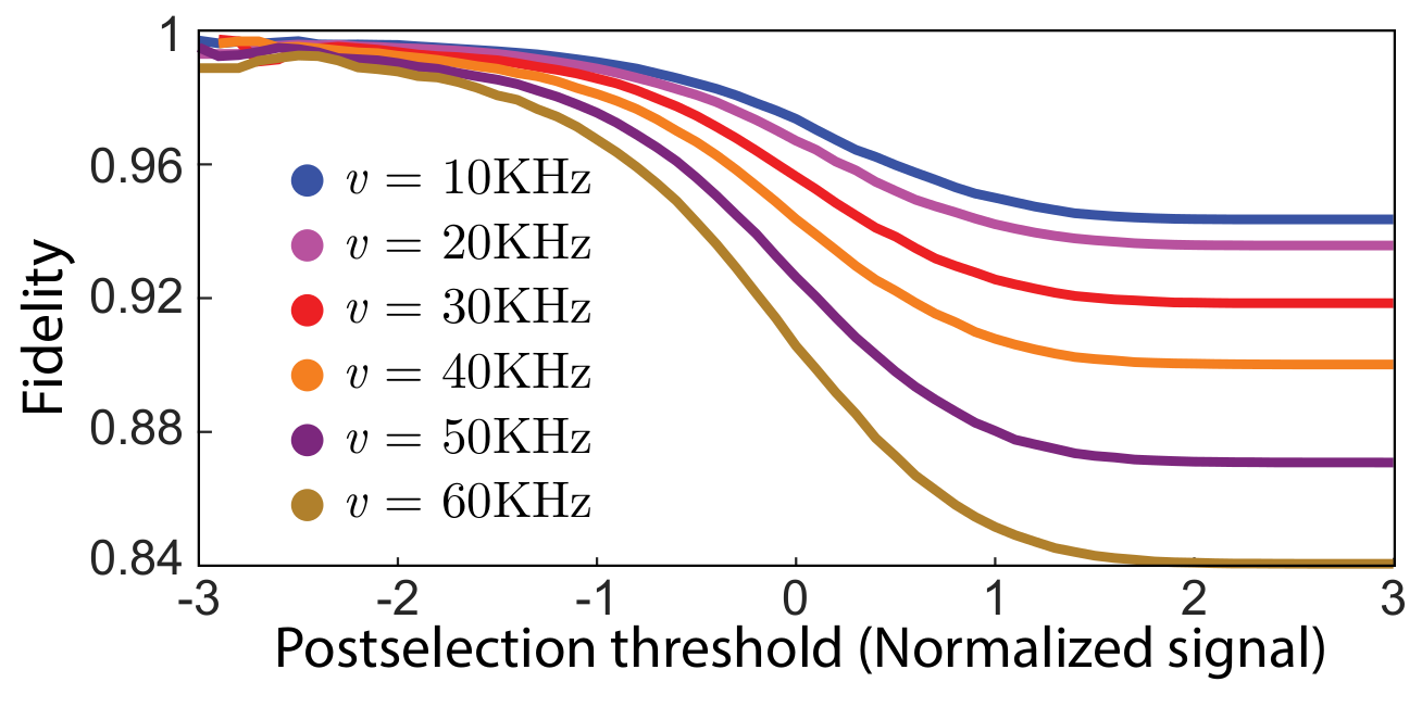
Post-selecting on trajectories with an average readout with a value >1 keeps only trajectories that did not jump, heralding a reasonably high-fidelity dragging gate for that subset
Alternatively, the jump may be observed, then corrected later

Result: Incoherent Qubit Gate using Quantum Zeno Effect
Siddiqi group, Nature 538, 491 (2016)
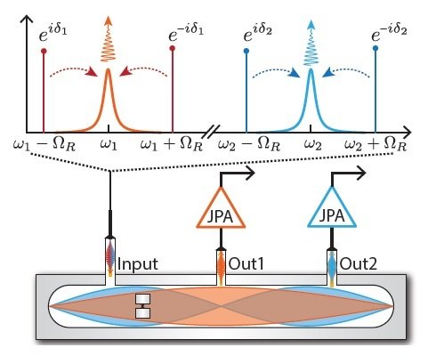
4 pumps, symmetrically detuned from
2 resonator modes of 3D transmon
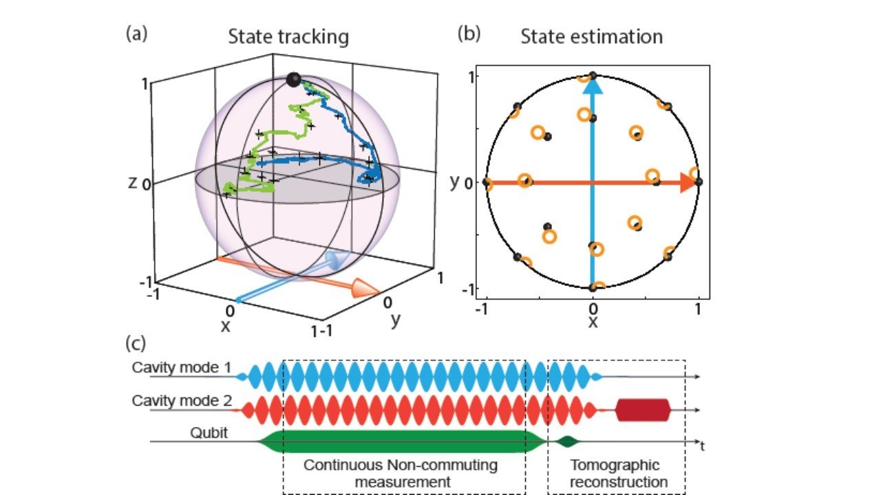
2 simultaneous noncommuting observables
Result : Simultaneous Noncommuting Observable Measurement
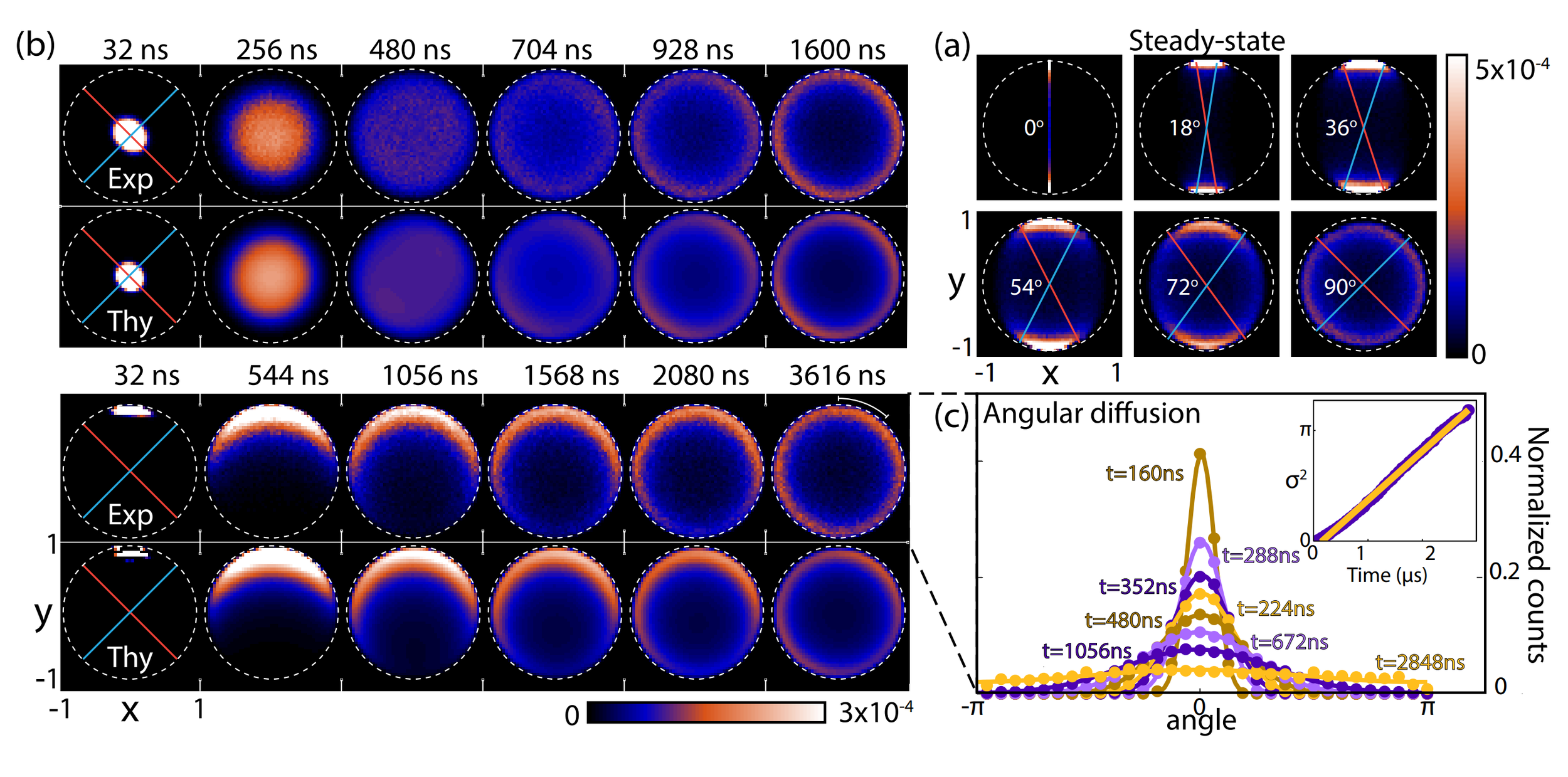
Siddiqi group, Nature 538, 491 (2016)
Observable incompatibility leads to diffusion around Bloch sphere
Result : Simultaneous Noncommuting Observable Measurement
Basins of attraction if measurement axes are nearly aligned
Tracking Quantum Jumps by Filtering Readout
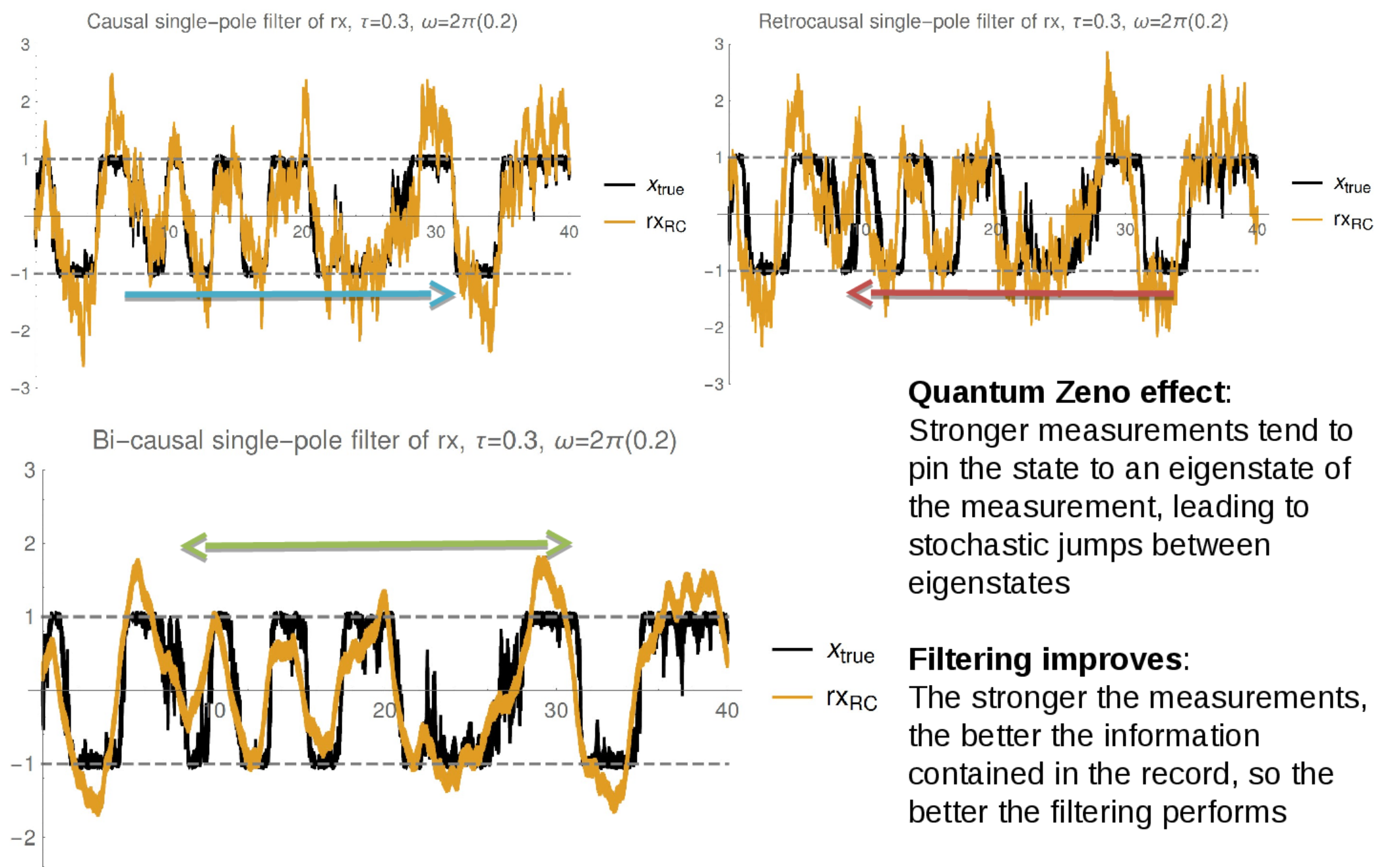
For stronger measurements: noise can be classically filtered to show qubit state
Useful for tracking the stochastic jumps between measurement eigenstates
Rabi drive, qubit oscillations:
Quantum Zeno regime:
Noisy qubit monitoring:
Tracking State with Noncommuting Observable Measurement
see also Ruskov et al. PRL 105 100506 (2010): >90% state fidelity with 3 axis monitoring + filtering
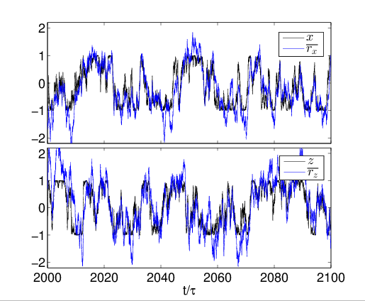
Observation: Since the readouts of each observable (here X and Z) follow the expectation values as they are causally generated, we can track the state using simple classical signal filtering
Left: causal exponential filter on readouts (blue) compared to actual simulated expectation values (black), showing reasonable fidelity tracking
This works because both measurements can be made sufficiently strong for information to be extracted within the averaging window of the filter
Crude state tomography with minimal priors
What is the limitation?
JD group, Phys. Rev. A 94, 062119 (2016)
If the collected stochastic signal noisily tracks an observable of the qubit, can we filter the signal to estimate that observable trajectory independently?
Idea: Readout-filtering for tomography
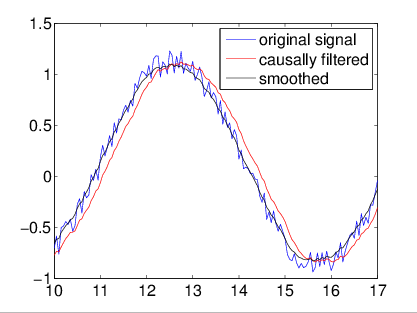
Classical signals can remove Gaussian noise either:
1)
Causally (no future signal), with a
filter (e.g. Weiner, Kalman)
2) Non-causally (using future signal), with a smoother
For already collected data, smoothers work best
Monitored qubit Z operator:
causally generated readout
Signal
Observ. Exp. Value
Gaussian Noise
Structure of collected qubit signal seems amenable to such a filtering technique
Filter independent of trajectory model
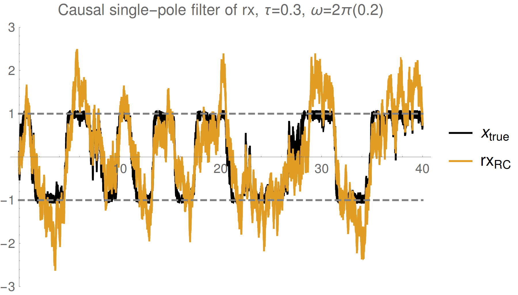
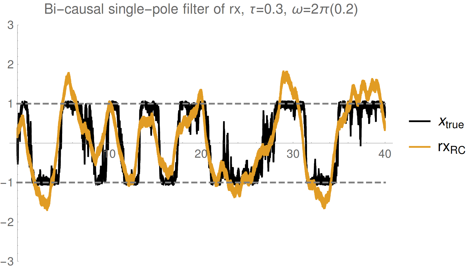
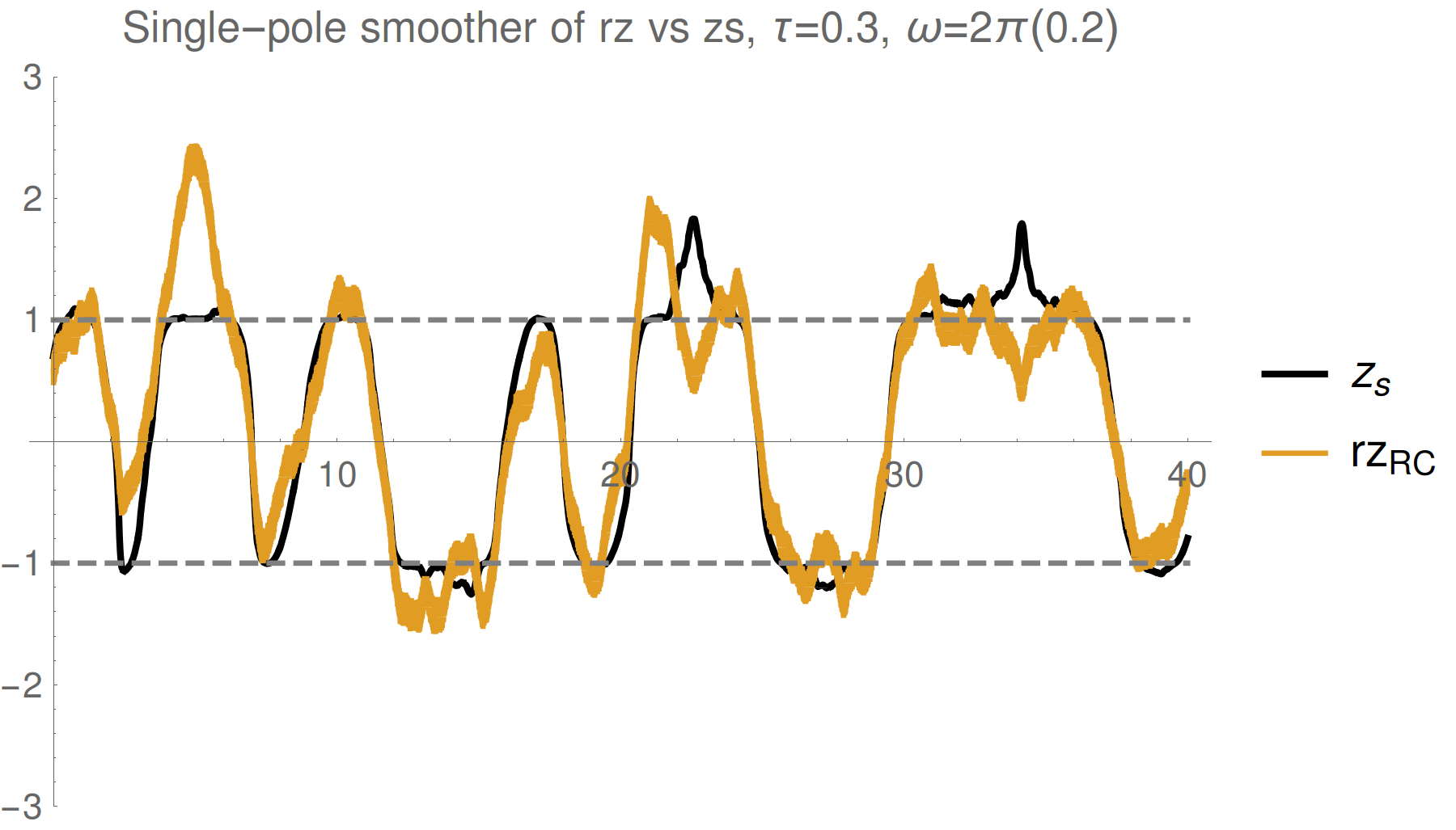
Simple single pole filter
Simple single pole smoother
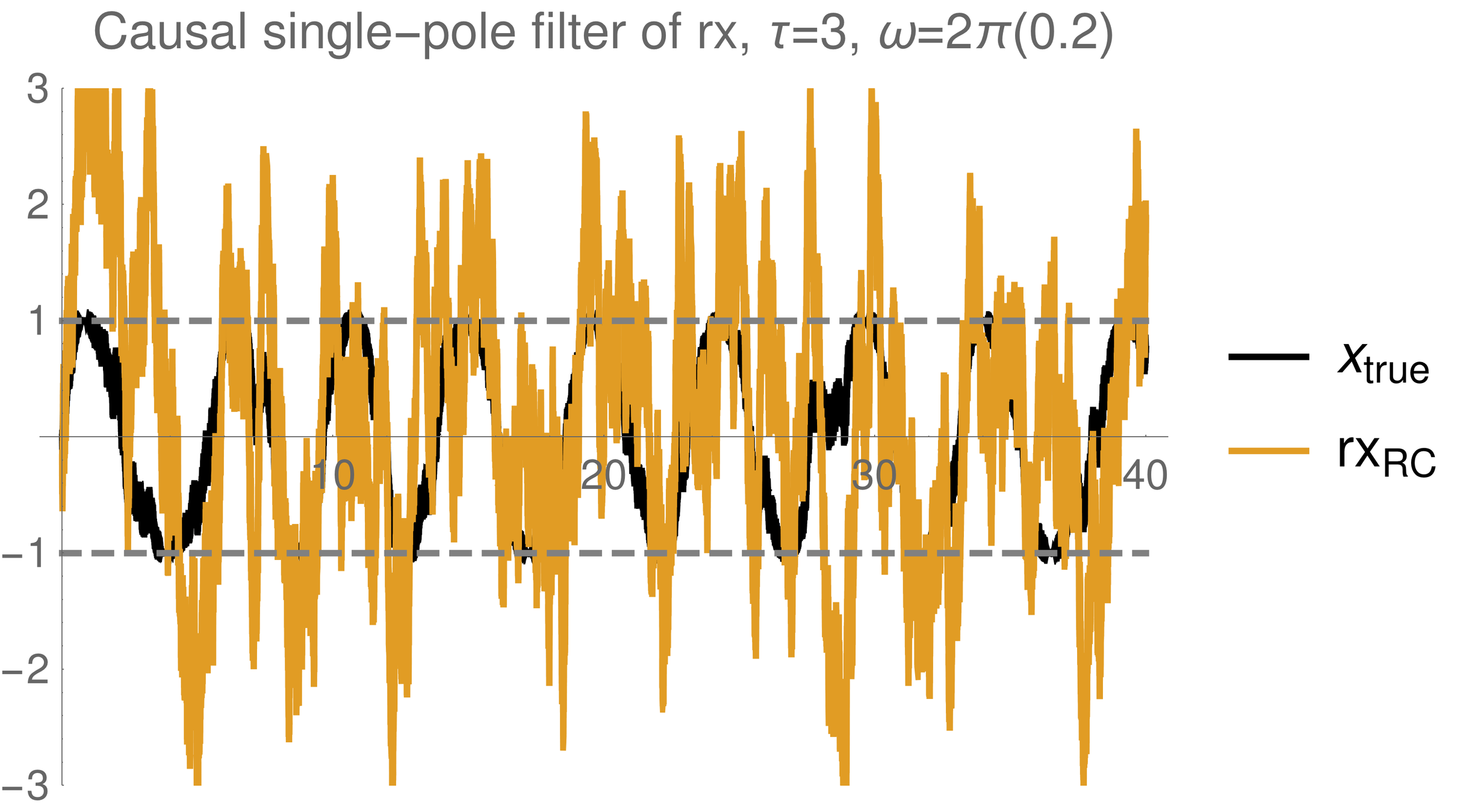
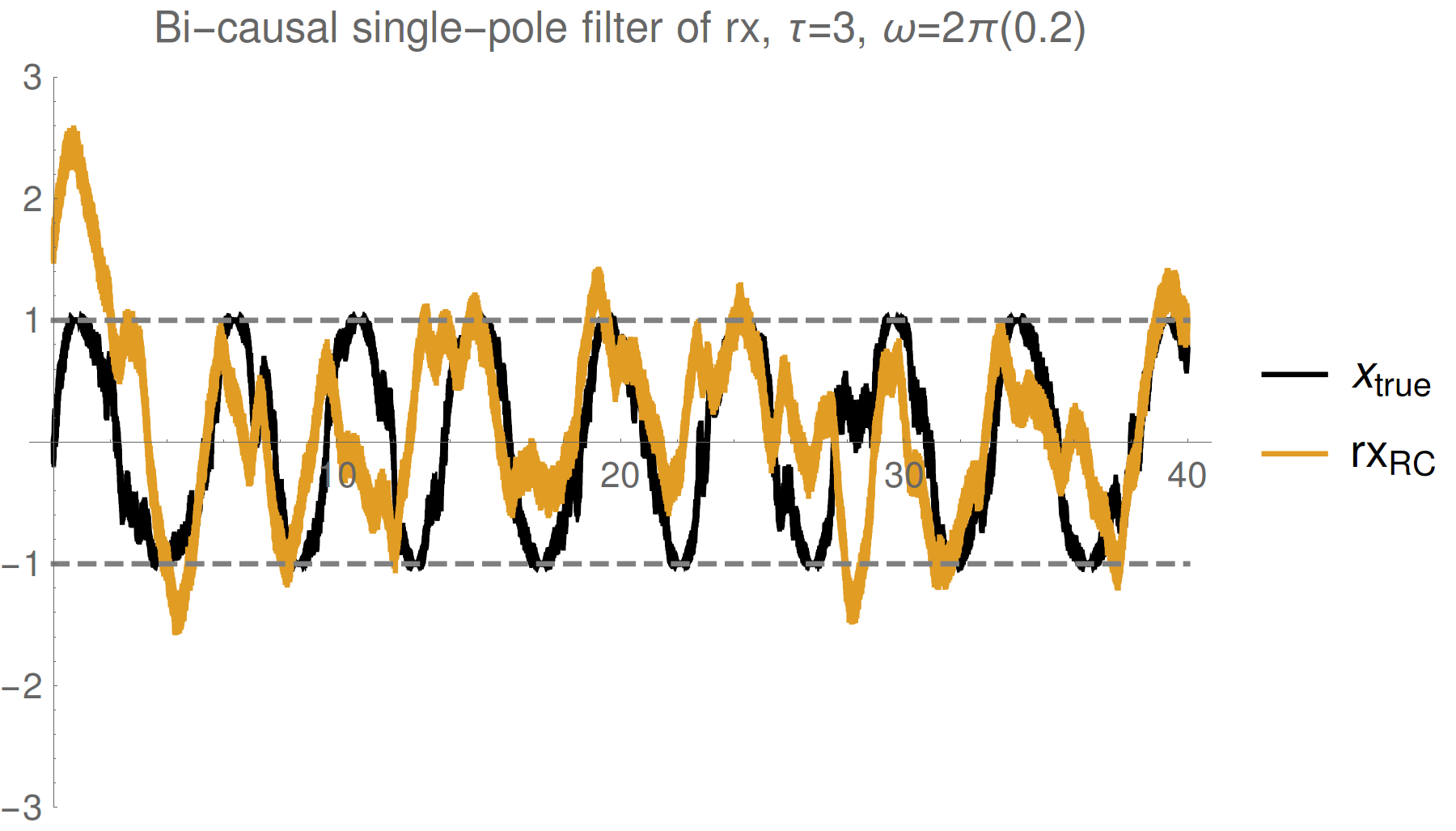
Strong (Zeno) regime: tracking jumps
Weak regime: tracking noisy Rabi oscillations
Trend : stronger measurements yield more information
--> better fidelity, but more perturbed evolution
Reasonable tracking
Noise harder to remove
Evidence: Readout-filtering for Zeno tracking
Consider a single collected readout r(t), but omit one point at t=tj.
What distribution P[r(tj)] describes the likelihood of the omitted point?
Result: Shifted Past Readout Distribution
Discretize time into bins of size dt - assume Markovian Gaussian measurements:
We recover approximate Gaussian noise, as expected:
However, the collected readout follows a shifted mean value
(Consequence of the measurement backaction producing non-Markovian correlations)
The mean is the expectation value of Z only on the boundary, with unknown future record (as appropriate for simulation)
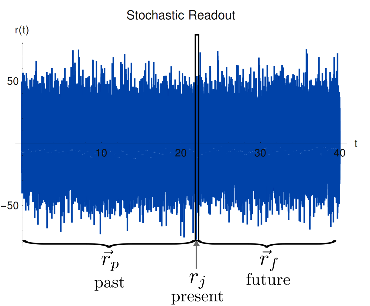
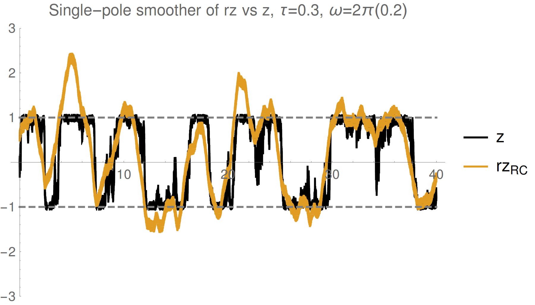

JD group, arXiv:1708.04362
Optimally filtering/smoothing a single collected readout
will remove the Gaussian noise, and recover the
shifted observable value, not the expectation value
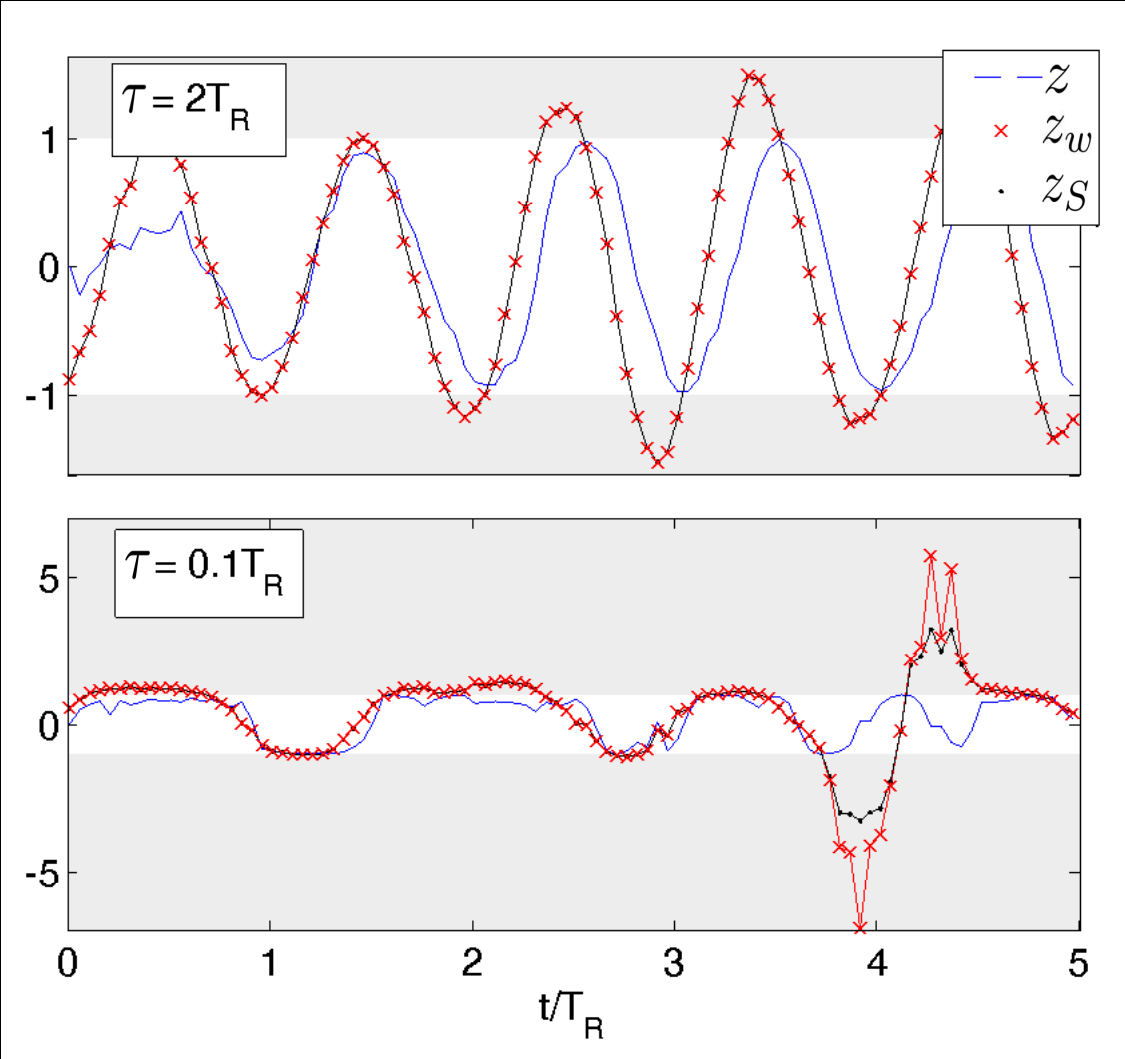
Weak regime
Strong regime
Smoothed (shifted) observable mean:
Depends on a weak value and a quadratric correction:
Non-Markovian dependence on both
past state and future effect matrix:
Consistent with:
Aharonov PRL 60, 1351 (1988), Wiseman PRA 65, 032111 (2002), Tsang PRL 102, 250403 (2009), Dressel PRL 104, 240401 (2010), Dressel PRA 88, 022107 (2013), Mølmer PRL 111, 160401 (2013)
( No additional ad hoc postselection)
Result: Smoothed Past Observable Estimate
JD group, arXiv:1708.04362
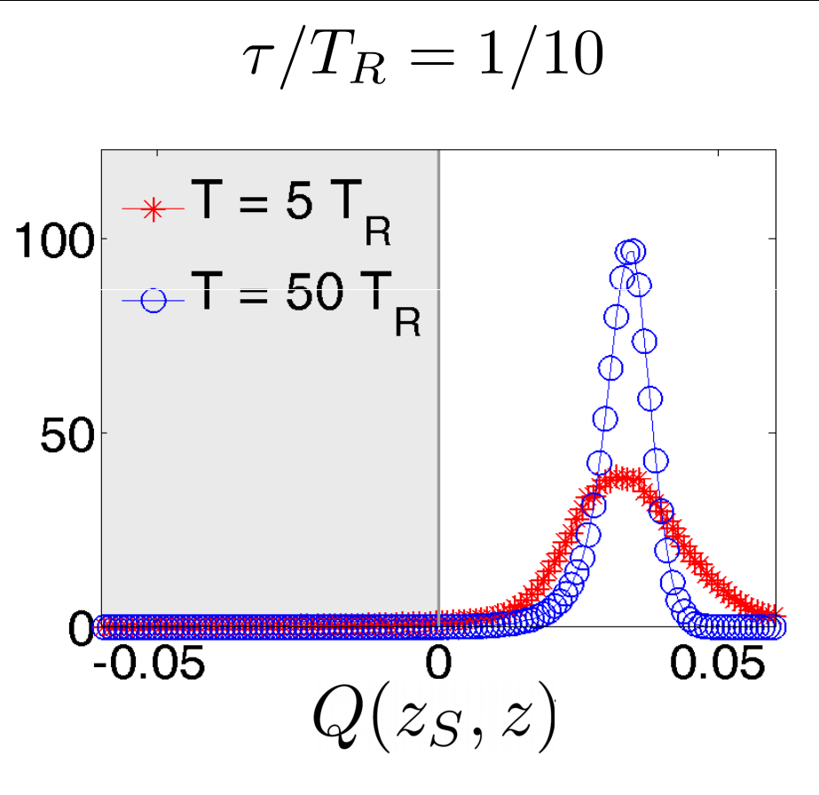
Is this really true? This smoothed value seems strange - can exceed eigenvalue range
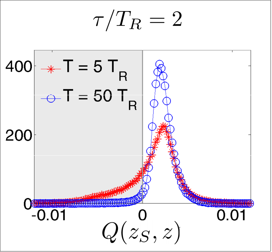
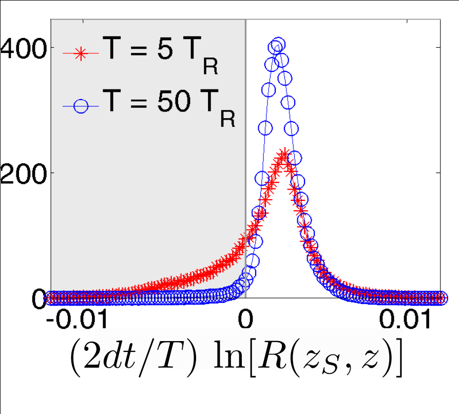
Verification 1: look at relative mean-squared error of
both estimates compared to raw readout
Optimal filters/smoothers (Weiner, Kalman, etc.) are often defined to minimize the MSE between a smooth dynamical estimate and the raw noisy signal
Discriminator:
(>0 implies smoothed value follows readout better than expectation value)
Strong regime
Weak regime
smoothed better

Yes. The smoothed value is objectively better by the same metric used for finding classical filters/smoothers.
Result: Smoothed Estimate minimizes MSE
JD group, arXiv:1708.04362
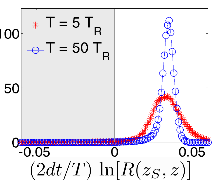
Verification 2: look at relative
log-likelihood of
generating the raw readout from adding Gaussian noise to the two estimates - equivalent to a hypothesis test
Discriminator:
(>0 implies smoothed value more likely than expectation value to generate readout)
Strong regime
Weak regime
smoothed better
Yes. The smoothed value is objectively more likely to generate the observed readout from additive noise


Result: Smoothed Estimate beats Hypothesis Test
JD group, arXiv:1708.04362
Variation: Suppose Bob is weakly monitoring a different observable (X) at the same time
If Alice is more strongly monitoring (Z) and has no access to Bob's record, does her smoothed estimate of X (not measured by her) still correspond to Bob's record?
Red : Alice does not know Bob's record, exp. val.
Black : Alice does not know Bob's record, smoothed
Blue : Alice knows both records, smoothed
smoothed better
[Similar question to Guevara, Wiseman PRL 115, 180407 (2015) ]

Result: Smoothed Estimate predicts 3rd Party measurement
Yes. Even without access to Bob's record, Alice can construct a smoothed estimate from her record that fits Bob's observed record better than even the expectation value constructed from perfect knowledge of both measurements
Smoothed estimate is operationally meaningful
JD group, arXiv:1708.04362
Conclusions


- Continuous measurements and quantum trajectories can now be used in the laboratory with superconducting transmon circuits
- 10+ qubit planar 2D transmon designs in-hand at UCB
- Both dispersive and displacement measurements are possible
- The quantum Zeno effect can be used to produce a heralded measurement-based qubit gate using time-dependent axes
- Multiple noncommuting observables can be measured simultaneously
- The stochastic readout collected from a qubit measurement approximates the qubit state for crude tomography, but actually follows a smoothed observable estimate
Thank you!
