Weak Values in the Wild

Justin Dressel
Institute for Quantum Studies, Chapman University

30th Anniversary of the Weak Value, 3/1/2018

Role 1 : Weak Values as multiplicative interaction parameters

Given a prepare-and-measure scenario, if an intermediate transformation is added then weak values completely determine the multiplicative correction to the amplitudes caused by the interaction.

\hat{U}_g = e^{-ig\hat{A}}

\hat{U}_g = e^{-ig\hat{A}}

\displaystyle \langle \phi | \hat{U}_g|\psi\rangle = \frac{\langle \phi | e^{-ig\hat{A}}|\psi\rangle}{\langle \phi | \psi \rangle} \langle \phi | \psi \rangle = \left[\sum_{n=0}^\infty (-ig)^n A_w^{(n)}\right] \langle \phi | \psi \rangle

\displaystyle \langle \phi | \hat{U}_g|\psi\rangle = \frac{\langle \phi | e^{-ig\hat{A}}|\psi\rangle}{\langle \phi | \psi \rangle} \langle \phi | \psi \rangle = \left[\sum_{n=0}^\infty (-ig)^n A_w^{(n)}\right] \langle \phi | \psi \rangle

|\psi\rangle

|\psi\rangle

\langle\phi |

\langle\phi |

Prepare

Transform

Measure

\displaystyle A_w^{(n)} \equiv \frac{\langle \phi | \hat{A}^n | \psi \rangle}{\langle \phi | \psi \rangle}

\displaystyle A_w^{(n)} \equiv \frac{\langle \phi | \hat{A}^n | \psi \rangle}{\langle \phi | \psi \rangle}

"Modular Value"

Multiplicative amplitude correction from

transformation

nth order "Weak Value"

Amplitude

Single System Weak Values

\hat{U}_g = e^{-ig\hat{A}\otimes\hat{B}}

\hat{U}_g = e^{-ig\hat{A}\otimes\hat{B}}

\displaystyle \langle \phi ,f| \hat{U}_g|\psi, i\rangle = \left[\sum_{n=0}^\infty (-ig)^n A_w^{(n)} B_w^{(n)}\right] \langle \phi | \psi \rangle \langle f | i \rangle

\displaystyle \langle \phi ,f| \hat{U}_g|\psi, i\rangle = \left[\sum_{n=0}^\infty (-ig)^n A_w^{(n)} B_w^{(n)}\right] \langle \phi | \psi \rangle \langle f | i \rangle

|\psi, i\rangle

|\psi, i\rangle

\langle\phi, f |

\langle\phi, f |

Prepare

Transform

Measure

Weak Coupling: Approximately first-order when g is small

\displaystyle \langle \phi ,f| \hat{U}_g|\psi, i\rangle \approx \left[1 -ig A_w B_w \right] \langle \phi | \psi \rangle \langle f | i \rangle \approx e^{-ig A_w B_w} \langle \phi | \psi \rangle \langle f | i \rangle

\displaystyle \langle \phi ,f| \hat{U}_g|\psi, i\rangle \approx \left[1 -ig A_w B_w \right] \langle \phi | \psi \rangle \langle f | i \rangle \approx e^{-ig A_w B_w} \langle \phi | \psi \rangle \langle f | i \rangle

System+Detector Weak Values

For detector momentum coupled to system :

A_w = \frac{\langle x | \hat{P} | \psi \rangle}{\langle x | \psi \rangle} = \frac{-i\partial_x\langle x | \psi \rangle}{\langle x | \psi \rangle} \Rightarrow \langle \phi ,f| \hat{U}_g|\psi, i\rangle \approx \left[1 -g B_w \partial_x \right] \langle x | \psi \rangle \langle f | i \rangle \approx e^{-g B_w \partial_x} \langle x | \psi \rangle \langle f | i \rangle = \langle x - g B_w | \psi \rangle \langle f | i \rangle

A_w = \frac{\langle x | \hat{P} | \psi \rangle}{\langle x | \psi \rangle} = \frac{-i\partial_x\langle x | \psi \rangle}{\langle x | \psi \rangle} \Rightarrow \langle \phi ,f| \hat{U}_g|\psi, i\rangle \approx \left[1 -g B_w \partial_x \right] \langle x | \psi \rangle \langle f | i \rangle \approx e^{-g B_w \partial_x} \langle x | \psi \rangle \langle f | i \rangle = \langle x - g B_w | \psi \rangle \langle f | i \rangle

Sagnac Beam-tilt Experiment

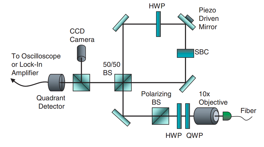
Howell lab, Rochester

PRL 102, 173601 (2009)

Ultra-sensitive to beam deflection: ~560 femto-radians of tilt detected

\phi\;\text{(phase offset)}

\phi\;\text{(phase offset)}

k\;\text{(tilt)}

k\;\text{(tilt)}

x\;\text{(signal)}

x\;\text{(signal)}

\sigma\;\text{(beam waist)}

\sigma\;\text{(beam waist)}

Collimated Beam Analysis

|i\rangle = \frac{i|\!\circlearrowleft\rangle + |\!\circlearrowright\rangle}{\sqrt{2}}

|i\rangle = \frac{i|\!\circlearrowleft\rangle + |\!\circlearrowright\rangle}{\sqrt{2}}

|f\rangle = \frac{e^{i\phi/2}|\!\circlearrowleft\rangle - ie^{-i\phi/2}|\!\circlearrowright\rangle}{\sqrt{2}}

|f\rangle = \frac{e^{i\phi/2}|\!\circlearrowleft\rangle - ie^{-i\phi/2}|\!\circlearrowright\rangle}{\sqrt{2}}

|\psi, i\rangle \to \langle x, f | \exp(-i k \hat{x}\hat{W}) | \psi, i \rangle = \langle x|\hat{M}_f\,|\psi\rangle = i\sin(\phi/2 - kx)\langle x | \psi\rangle

|\psi, i\rangle \to \langle x, f | \exp(-i k \hat{x}\hat{W}) | \psi, i \rangle = \langle x|\hat{M}_f\,|\psi\rangle = i\sin(\phi/2 - kx)\langle x | \psi\rangle

\hat{W} = |\!\circlearrowleft\rangle\langle\!\circlearrowleft\! | - |\!\circlearrowright\rangle\langle\!\circlearrowright\! |

\hat{W} = |\!\circlearrowleft\rangle\langle\!\circlearrowleft\! | - |\!\circlearrowright\rangle\langle\!\circlearrowright\! |

\phi\;\text{(phase offset)}

\phi\;\text{(phase offset)}

k\;\text{(tilt)}

k\;\text{(tilt)}

x\;\text{(signal)}

x\;\text{(signal)}

\sigma\;\text{(beam waist)}

\sigma\;\text{(beam waist)}

\hat{M}_f = \langle f | \exp(-i k \hat{x}\hat{W}) | i \rangle = i \sin(\phi/2 - k\hat{x})

\hat{M}_f = \langle f | \exp(-i k \hat{x}\hat{W}) | i \rangle = i \sin(\phi/2 - k\hat{x})

P(x) = |\langle x,f| \psi,i\rangle|^2 = \sin^2(\phi/2 - kx)\,P_0(x) = \frac{\sin^2(\phi/2 - kx)}{\sqrt{2\pi\sigma^2}} e^{-(x/\sigma)^2/2}

P(x) = |\langle x,f| \psi,i\rangle|^2 = \sin^2(\phi/2 - kx)\,P_0(x) = \frac{\sin^2(\phi/2 - kx)}{\sqrt{2\pi\sigma^2}} e^{-(x/\sigma)^2/2}

Original profile of beam becomes modulated.

JD et al., PRA 88 , 023801 (2013)

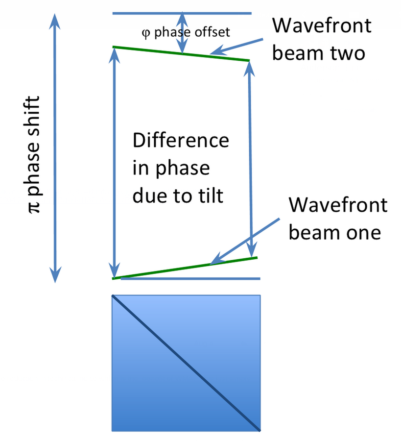
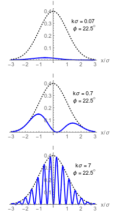
Collimated Dark Port Profiles

Left: Wavefront tilt mechanism producing spatial modulation

Right: Asymmetric dark port profiles in different regimes

Dashed envelope: input beam intensity

Solid curve:

dark port intensity

Top right:

weak value regime

Middle right:

double lobe regime

Bottom right:

misaligned regime

k\sigma \ll \phi \ll 1

k\sigma \ll \phi \ll 1

\phi\ll k\sigma \ll 1

\phi\ll k\sigma \ll 1

\phi\ll 1 \ll k\sigma

\phi\ll 1 \ll k\sigma

Weak Value Analysis

|i\rangle \propto i|\!\circlearrowleft\rangle + |\!\circlearrowright\rangle

|i\rangle \propto i|\!\circlearrowleft\rangle + |\!\circlearrowright\rangle

|f\rangle \propto e^{i\phi/2}|\!\circlearrowleft\rangle - ie^{-i\phi/2}|\!\circlearrowright\rangle

|f\rangle \propto e^{i\phi/2}|\!\circlearrowleft\rangle - ie^{-i\phi/2}|\!\circlearrowright\rangle

|\psi, i\rangle \to \langle p, f | \exp(-i k \hat{x}\hat{W}) | \psi, i \rangle \approx \langle f | i \rangle \langle p - k W_w | \psi \rangle

|\psi, i\rangle \to \langle p, f | \exp(-i k \hat{x}\hat{W}) | \psi, i \rangle \approx \langle f | i \rangle \langle p - k W_w | \psi \rangle

\hat{W} = |\!\circlearrowleft\rangle\langle\!\circlearrowleft | - |\!\circlearrowright\rangle\langle\!\circlearrowright |

\hat{W} = |\!\circlearrowleft\rangle\langle\!\circlearrowleft | - |\!\circlearrowright\rangle\langle\!\circlearrowright |

W_w = \frac{\langle f |\hat{W}|i\rangle}{\langle f | i \rangle} = i\cot\frac{\phi}{2} \approx \frac{2i}{\phi}

W_w = \frac{\langle f |\hat{W}|i\rangle}{\langle f | i \rangle} = i\cot\frac{\phi}{2} \approx \frac{2i}{\phi}

\phi\;\text{(phase offset)}

\phi\;\text{(phase offset)}

k\;\text{(tilt)}

k\;\text{(tilt)}

x\;\text{(signal)}

x\;\text{(signal)}

\sigma\;\text{(beam waist)}

\sigma\;\text{(beam waist)}

Angular tilt (transverse momentum) amplified by large weak value.

Weak value regime

k\sigma \ll \phi \ll 1

k\sigma \ll \phi \ll 1

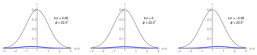
Dark port has single lobe that approximates a displaced Gaussian centered at:

\langle x/\sigma \rangle \propto (\mathbf{k}/\phi)\sigma

\langle x/\sigma \rangle \propto (\mathbf{k}/\phi)\sigma

Tiny beam deflections can be distinguished, but with low output intensity.

I \propto \phi^2

I \propto \phi^2

Role 2 : Weak Values as minimum error estimations

Given a known preparation and postselection, the real part of a weak value is the best estimate of an unknown observable value in between.

\mathcal{D}_\psi (\hat{A},\hat{B}) = \langle\psi |(\hat{A} - \hat{B})^2 |\psi\rangle

\mathcal{D}_\psi (\hat{A},\hat{B}) = \langle\psi |(\hat{A} - \hat{B})^2 |\psi\rangle

Consider a distance measure between two observables (mean-squared "operator error"):

Suppose you wish to estimate \(\hat{A}\), but measure a basis \(\{|f\rangle\}\) that is not its eigenbasis. What is the closest observable to \(\hat{A}\) that you can estimate? That is, what values \(\bar{a}_f\) should you assign to each observed outcome to minimize the operator error?

\hat{A}_{\text{est}} = \sum_f \bar{a}_f |f\rangle\langle f|

\hat{A}_{\text{est}} = \sum_f \bar{a}_f |f\rangle\langle f|

\mathcal{D}_\psi(\hat{A},\hat{A}_{\text{est}}) = \langle \psi | \hat{A}^2 | \psi\rangle - \sum_f |\langle f | \psi \rangle |^2 \left[\text{Re}\frac{\langle f | \hat{A} | \psi \rangle}{\langle f | \psi \rangle}\right]^2 + \sum_f |\langle f | \psi \rangle | ^2 \left[ \bar{a}_f - \text{Re}\frac{\langle f | \hat{A} | \psi\rangle}{\langle f | \psi \rangle}\right]^2

\mathcal{D}_\psi(\hat{A},\hat{A}_{\text{est}}) = \langle \psi | \hat{A}^2 | \psi\rangle - \sum_f |\langle f | \psi \rangle |^2 \left[\text{Re}\frac{\langle f | \hat{A} | \psi \rangle}{\langle f | \psi \rangle}\right]^2 + \sum_f |\langle f | \psi \rangle | ^2 \left[ \bar{a}_f - \text{Re}\frac{\langle f | \hat{A} | \psi\rangle}{\langle f | \psi \rangle}\right]^2

Only dependence on estimated values

Conclusion: the real part of the weak value is the best estimate for an observable value given the known boundary conditions

\bar{a}_f = \text{Re}\frac{\langle f | \hat{A} | \psi \rangle}{\langle f | \psi \rangle}

\bar{a}_f = \text{Re}\frac{\langle f | \hat{A} | \psi \rangle}{\langle f | \psi \rangle}

\hat{Z} = |1\rangle\langle 1 | - |0\rangle\langle 0|

\hat{Z} = |1\rangle\langle 1 | - |0\rangle\langle 0|

|\psi \rangle = |1\rangle

|\psi \rangle = |1\rangle

\langle f | = \langle 0 |

\langle f | = \langle 0 |

\displaystyle \hat{H} = \frac{\omega}{2} \left( |1\rangle\langle 0| + |0\rangle\langle 1|\right)

\displaystyle \hat{H} = \frac{\omega}{2} \left( |1\rangle\langle 0| + |0\rangle\langle 1|\right)

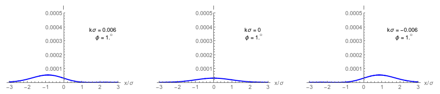
Evolving Best Estimate

Whenever the observable is an eigenvalue with certainty, the weak value must match.

If the evolution is not consistent with the boundary conditions, then the weak value smoothly interpolates while preserving both the certainty of the eigenvalues and the periodicity of the evolution.

What information is contained in the noisy voltage signal obtained while measuring quantum state trajectories?

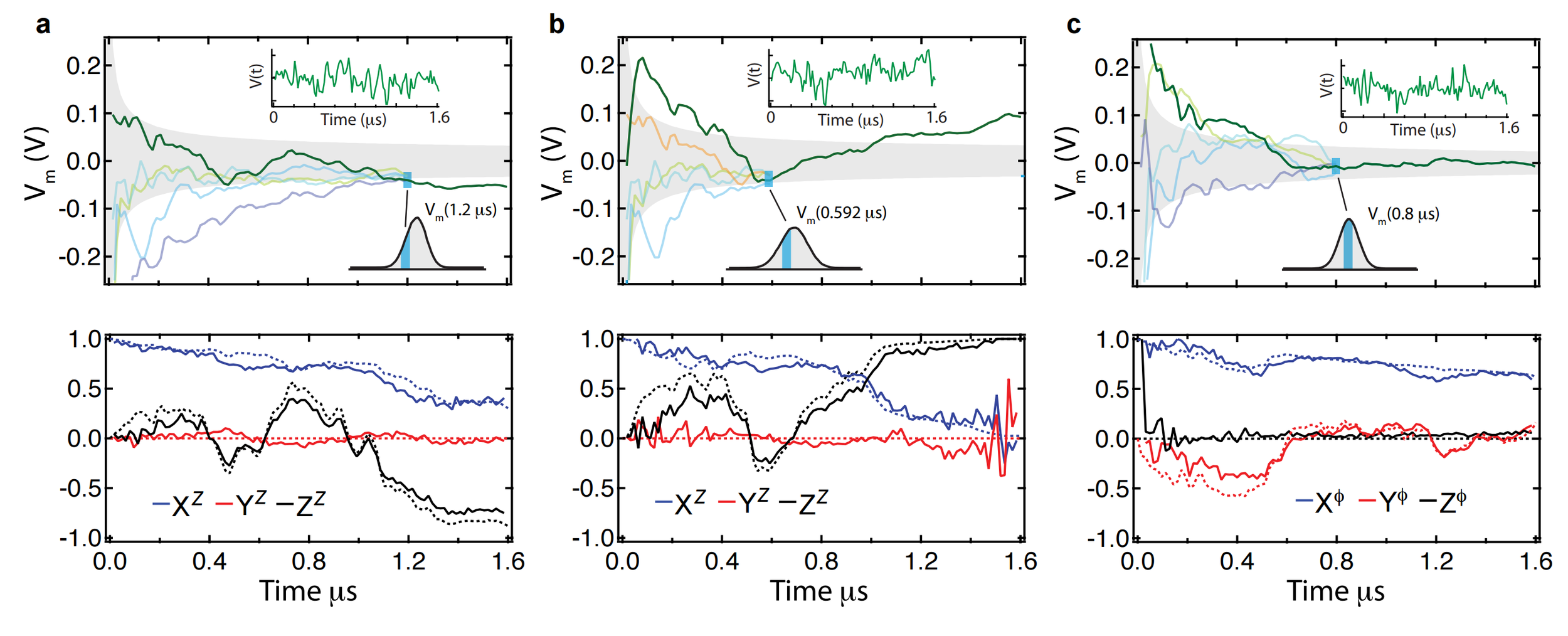
Continuous Monitoring Example

Murch et al., Nature 502, 211 (2013)

Hacohen-Gourgy et al., Nature 538, 491 (2016)

If the collected stochastic signal noisily tracks an observable of the qubit, can we filter the signal to estimate that observable trajectory independently?

Idea: Filter the Readout

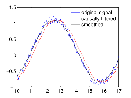
Classical signals can remove Gaussian noise either:

1) Causally (no future signal), with a filter (e.g. Weiner, Kalman)

2) Non-causally (using future signal), with a smoother

For already collected data, smoothers work best

r(t) = z(t) + \sqrt{\tau}\,\xi(t)

r(t) = z(t) + \sqrt{\tau}\,\xi(t)

Monitored qubit Z operator:

causally generated readout

Signal

Observ. Exp. Value

Gaussian Noise

Structure of collected qubit signal seems amenable to such a filtering technique

Filter independent of trajectory model

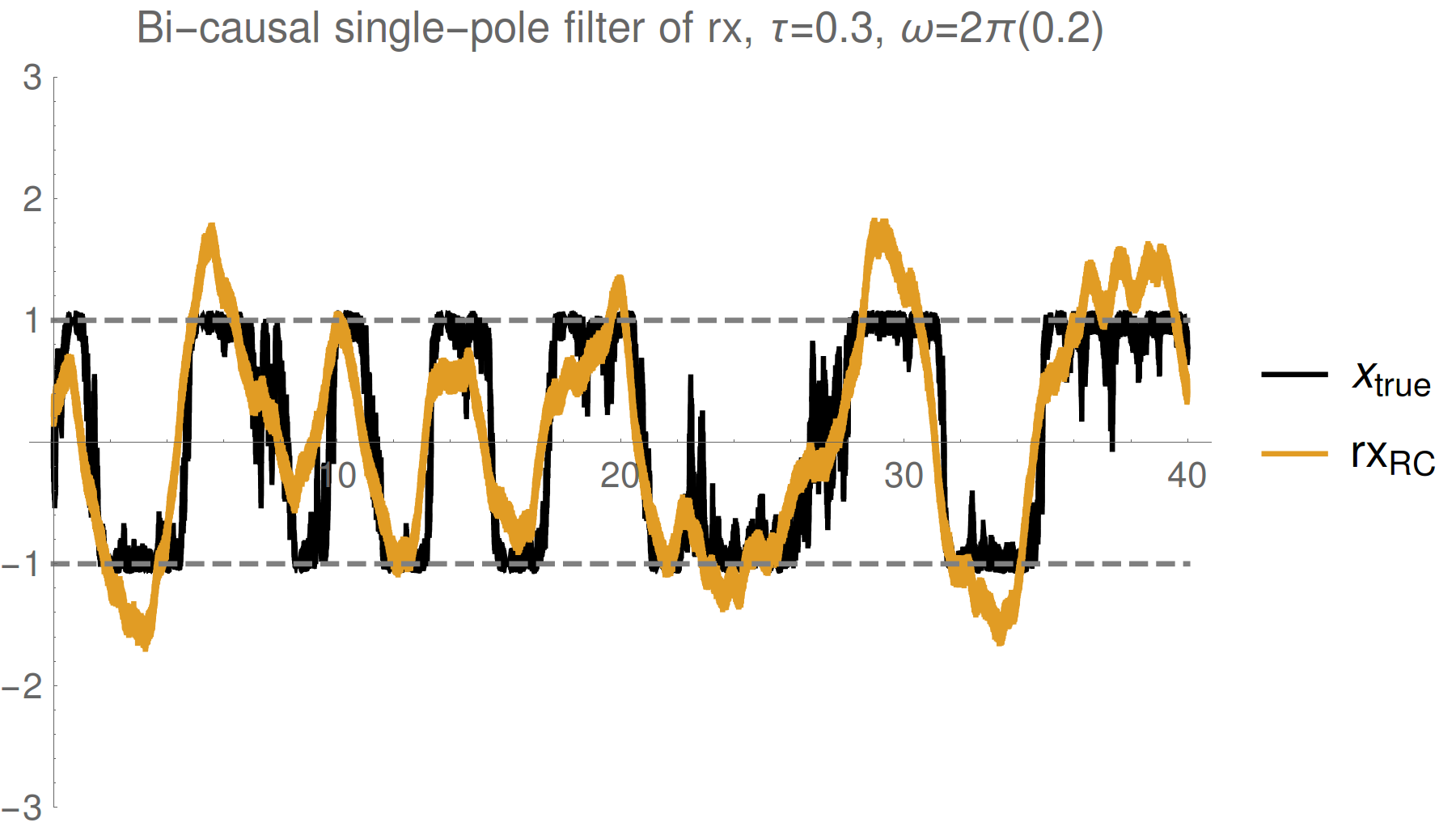
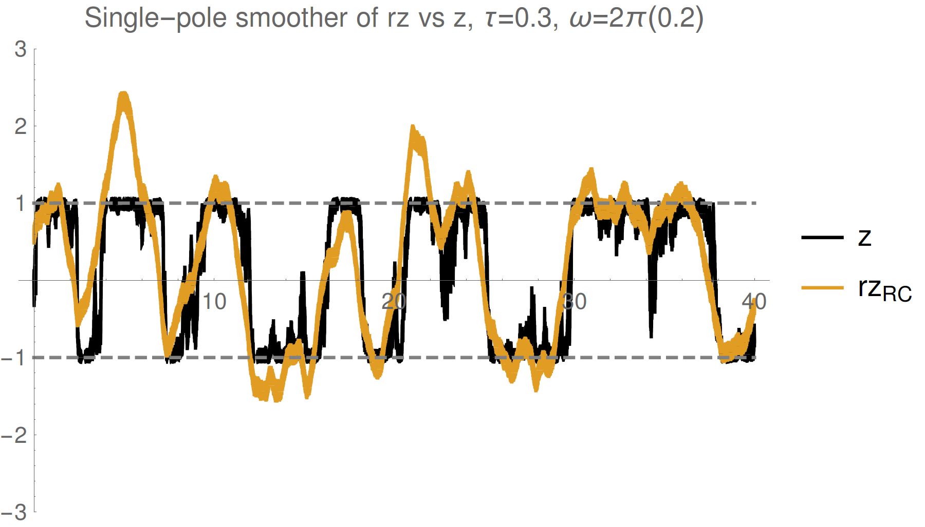
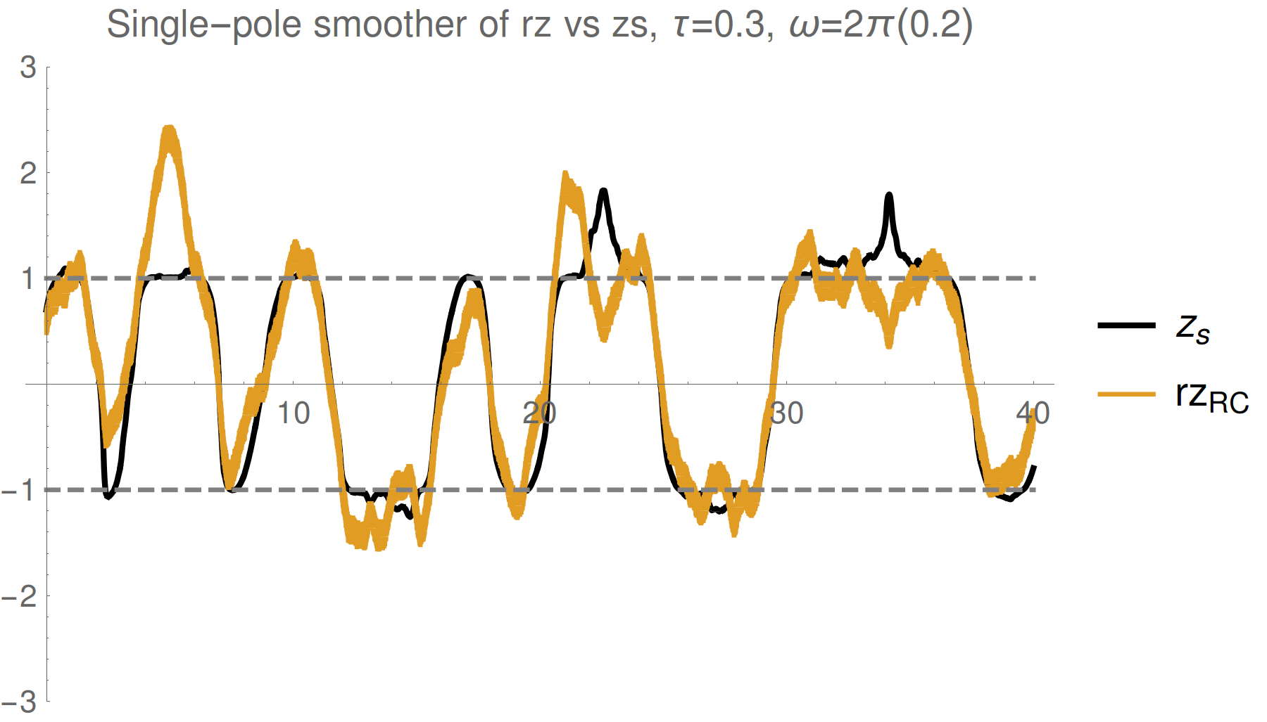
z(t) = \mathrm{Tr}[Z\,\rho_{\vec{r}_{\mathrm{past}}}]

z(t) = \mathrm{Tr}[Z\,\rho_{\vec{r}_{\mathrm{past}}}]

Example : Qubit Z

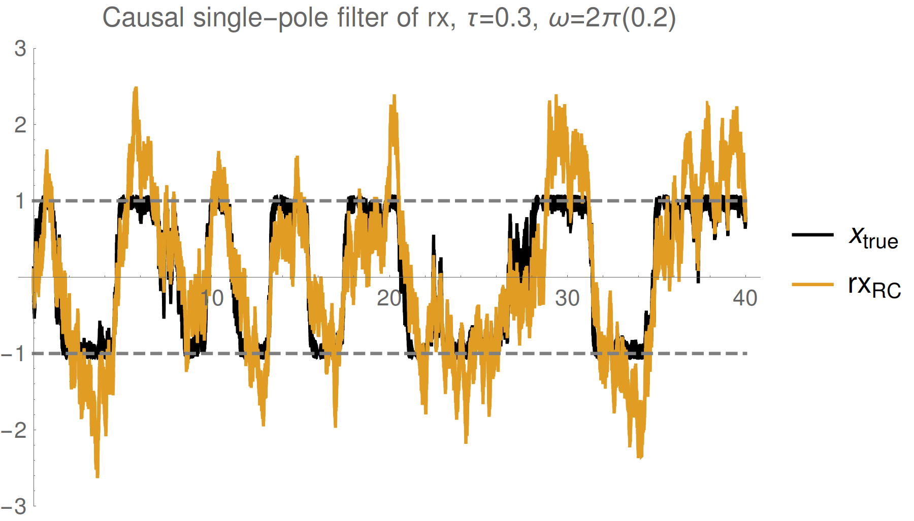
Simple single pole filter

Simple single pole smoother

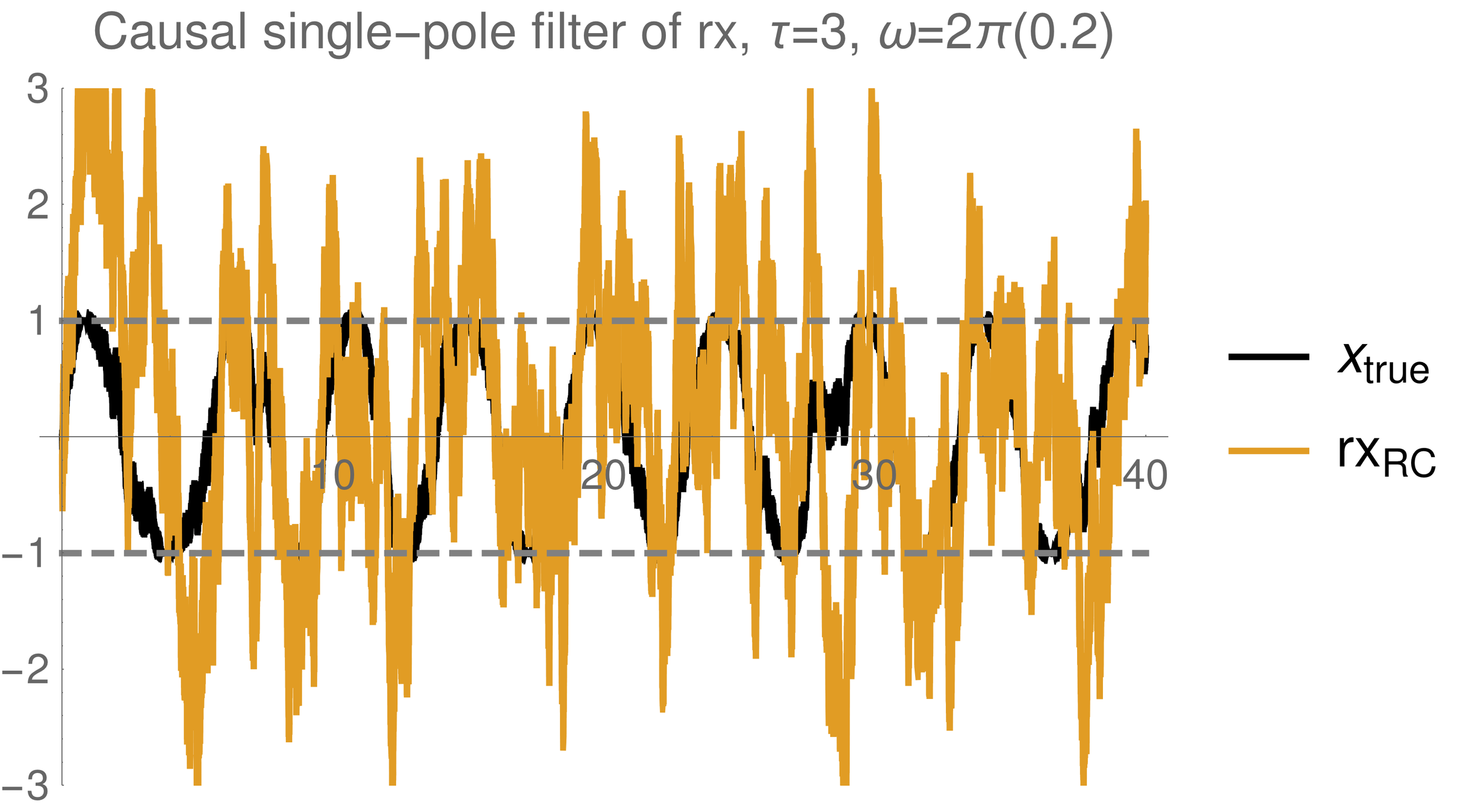
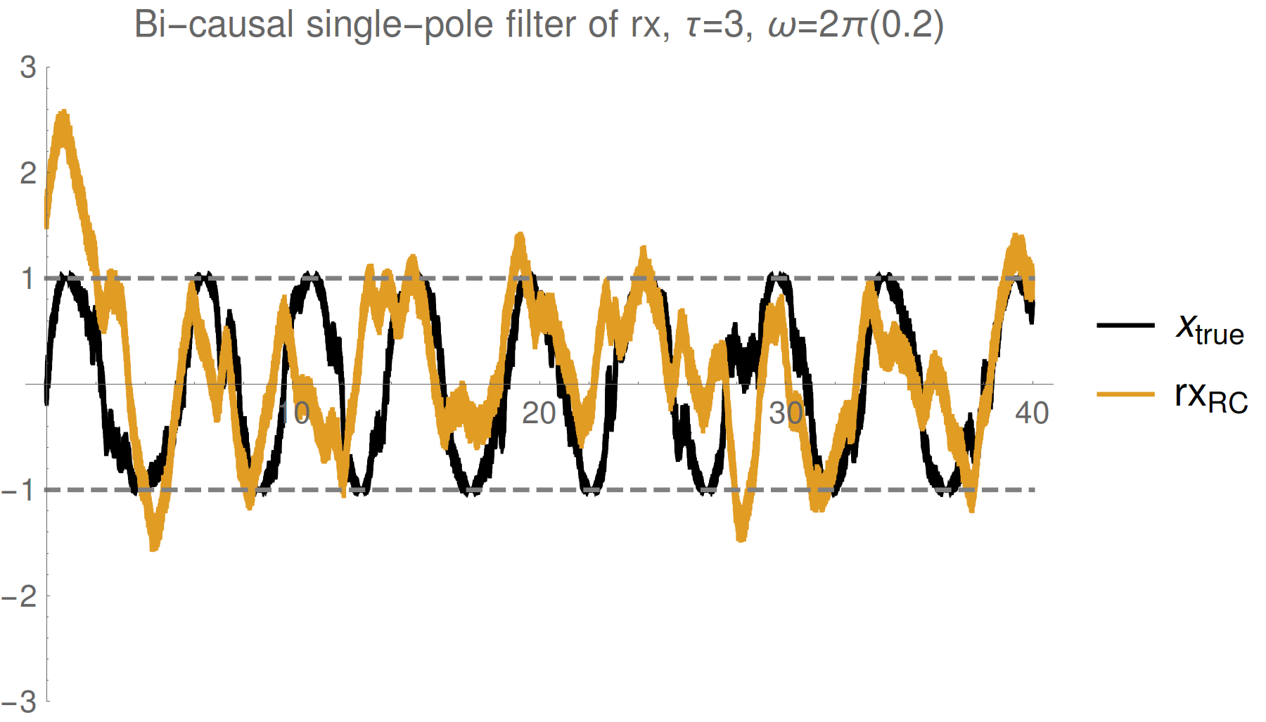
Strong (Zeno) regime: tracking jumps

Weak regime: tracking noisy Rabi oscillations

Trend : stronger measurements yield more information

--> better fidelity, but more perturbed evolution

Reasonable tracking

Noise harder to remove

Consider a single collected readout r(t), but omit one point at t=t1.

What distribution P[r(t1)] describes the likelihood of the omitted point?

Past Readout Distribution

P(r\, |\, \vec{r}_{\mathrm{past}},\, \vec{r}_{\mathrm{future}}) = \frac{P(r,\, \vec{r}_{\mathrm{future}}\,|\,\vec{r}_{\mathrm{past}})}{\sum_r P(r,\, \vec{r}_{\mathrm{future}}\,|\,\vec{r}_{\mathrm{past}})} \approx \frac{\exp\left[-\frac{dt}{2\tau}(r-z_s)^2\right]}{\sqrt{2\pi\tau/dt}}

P(r\, |\, \vec{r}_{\mathrm{past}},\, \vec{r}_{\mathrm{future}}) = \frac{P(r,\, \vec{r}_{\mathrm{future}}\,|\,\vec{r}_{\mathrm{past}})}{\sum_r P(r,\, \vec{r}_{\mathrm{future}}\,|\,\vec{r}_{\mathrm{past}})} \approx \frac{\exp\left[-\frac{dt}{2\tau}(r-z_s)^2\right]}{\sqrt{2\pi\tau/dt}}

Discretize time into bins of size dt - assume Markovian Gaussian measurements:

We recover approximate Gaussian noise, as expected:

r(t) = z_s(t) + \sqrt{\tau}\,\xi(t)

r(t) = z_s(t) + \sqrt{\tau}\,\xi(t)

However, the collected readout follows a shifted mean value

(Consequence of the measurement backaction producing non-Markovian correlations)

The mean is the expectation value of Z only on the boundary, with unknown future record (as appropriate for simulation)

Smoothed Observable Estimate

r(t) = z_s(t) + \sqrt{\tau}\,\xi(t)

r(t) = z_s(t) + \sqrt{\tau}\,\xi(t)

Optimally filtering/smoothing a single collected readout

will remove the Gaussian noise, and recover the

shifted observable value, not the expectation value

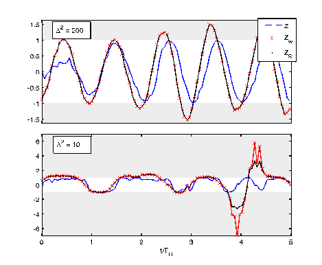
z_s = z_w\, \left[\frac{2}{(1+e^{-dt/2\tau}) + z_c\,(1-e^{-dt/2\tau})}\right] \approx z_w

z_s = z_w\, \left[\frac{2}{(1+e^{-dt/2\tau}) + z_c\,(1-e^{-dt/2\tau})}\right] \approx z_w

Weak regime

Strong regime

\displaystyle z_w = \mathrm{Re}\frac{\mathrm{Tr}[E_{\vec{r}_{\mathrm{future}}}\,Z\,\rho_{\vec{r}_{\mathrm{past}}}]}{\mathrm{Tr}[E_{\vec{r}_{\mathrm{future}}}\,\rho_{\vec{r}_{\mathrm{past}}}]}

\displaystyle z_w = \mathrm{Re}\frac{\mathrm{Tr}[E_{\vec{r}_{\mathrm{future}}}\,Z\,\rho_{\vec{r}_{\mathrm{past}}}]}{\mathrm{Tr}[E_{\vec{r}_{\mathrm{future}}}\,\rho_{\vec{r}_{\mathrm{past}}}]}

Smoothed (shifted) observable mean:

Depends on a weak value and a quadratric correction:

\displaystyle z_c = \frac{\mathrm{Tr}[E_{\vec{r}_{\mathrm{future}}}\,Z\,\rho_{\vec{r}_{\mathrm{past}}}\,Z]}{\mathrm{Tr}[E_{\vec{r}_{\mathrm{future}}}\,\rho_{\vec{r}_{\mathrm{past}}}]}

\displaystyle z_c = \frac{\mathrm{Tr}[E_{\vec{r}_{\mathrm{future}}}\,Z\,\rho_{\vec{r}_{\mathrm{past}}}\,Z]}{\mathrm{Tr}[E_{\vec{r}_{\mathrm{future}}}\,\rho_{\vec{r}_{\mathrm{past}}}]}

\rho_{\vec{r}_{\mathrm{past}}} = \mathcal{M}_{\vec{r}_{\mathrm{past}}}[\rho_0]

\rho_{\vec{r}_{\mathrm{past}}} = \mathcal{M}_{\vec{r}_{\mathrm{past}}}[\rho_0]

E_{\vec{r}_{\mathrm{future}}} = \mathcal{M}^*_{\vec{r}_{\mathrm{future}}}[1]

E_{\vec{r}_{\mathrm{future}}} = \mathcal{M}^*_{\vec{r}_{\mathrm{future}}}[1]

Non-Markovian dependence on both

past state and future effect matrix:

Consistent with:

Aharonov PRL 60, 1351 (1988), Wiseman PRA 65, 032111 (2002), Tsang PRL 102, 250403 (2009), Dressel PRL 104, 240401 (2010), Dressel PRA 88, 022107 (2013), Mølmer PRL 111, 160401 (2013)

( No additional ad hoc postselection)

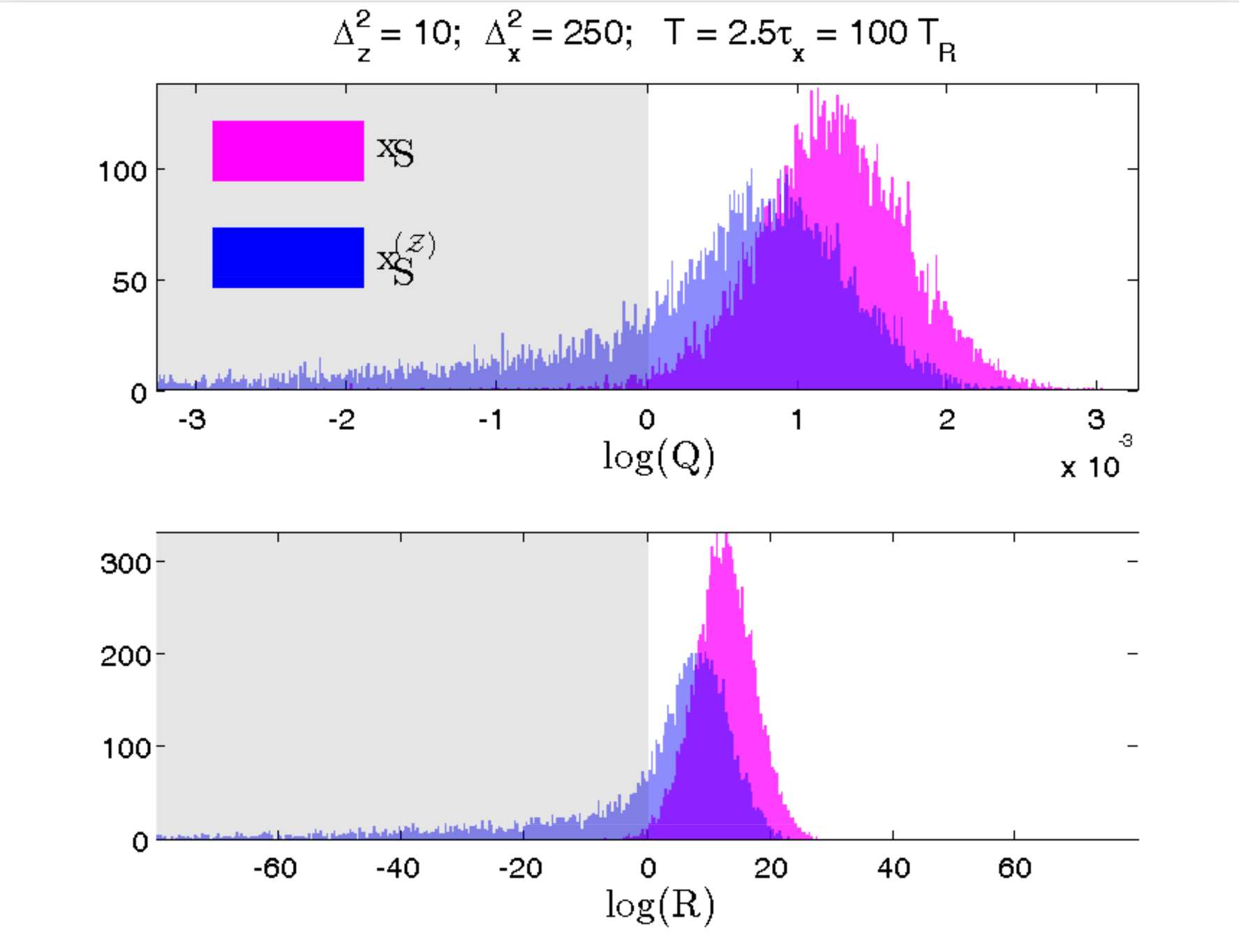
Reduced RMS Error from Readout

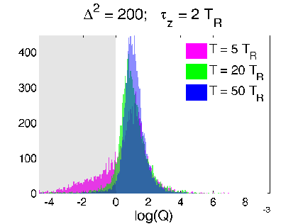
Is this really true? The estimate is a weak value that can exceed eigenvalue range

Verification 1: look at relative RMS error of
both estimates compared to raw readout

Optimal filters/smoothers (Weiner, Kalman, etc.) are often defined to minimize the RMS error between a smooth dynamical estimate and the raw noisy signal

\displaystyle \log(Q) \equiv \log\frac{||z - r||}{||z_s - r||}

\displaystyle \log(Q) \equiv \log\frac{||z - r||}{||z_s - r||}

Discriminator:
(>0 implies smoothed value follows readout better than expectation value)

T_R : \mathrm{Rabi\, period}

T_R : \mathrm{Rabi\, period}

\Delta^2 : \tau_z/dt

\Delta^2 : \tau_z/dt

Strong regime

Weak regime

T : \mathrm{traj.\,length}

T : \mathrm{traj.\,length}

smoothed better

Yes. The smoothed value is objectively better by the same metric used for finding classical filters/smoothers.

Hypothesis Test from Readout

Verification 2: look at relative log-likelihood of
generating the raw readout from adding Gaussian noise to the two estimates - equivalent to a hypothesis test

\displaystyle \log(R) \equiv \log\frac{P(r|z)}{P(r|z_s)}

\displaystyle \log(R) \equiv \log\frac{P(r|z)}{P(r|z_s)}

Discriminator:
(>0 implies smoothed value more likely than expectation value to generate readout)

T_R : \mathrm{Rabi\, period}

T_R : \mathrm{Rabi\, period}

\Delta^2 : \tau_z/dt

\Delta^2 : \tau_z/dt

Strong regime

Weak regime

T : \mathrm{traj.\,length}

T : \mathrm{traj.\,length}

smoothed better

Yes. The smoothed value is objectively more likely to generate the observed readout from additive noise

z

z_s

z_s

Corroboration by Third Party

Variation: Suppose Bob is weakly monitoring a different observable (X) at the same time

If Alice is more strongly monitoring (Z) and has no access to Bob's record, does her smoothed estimate of X (not measured by her) still correspond to Bob's record?

Yes. Even without access to Bob's record, Alice can construct a smoothed estimate from her record that fits Bob's observed record better than the expectation value (computed either from Alice's subjective state or the most pure state with perfect knowledge of both records)

Test verifies that a better model of the relevant dynamics produces an objectively closer fit to the collected record

Smoothed estimate is operationally meaningful

RMS Error Test

Hypothesis Test

Blue : Alice does not know Bob's record

Pink : Alice knows both records

smoothed better

[Similar question to Guevara, Wiseman PRL 115, 180407 (2015) ]

Role 3 : Weak Values as eigenvalue shifts

In spectroscopy, if a perturbation is added to the system, the energy spectra will shift by weak values of the perturbation.

\hat{H}|E_k\rangle = E_k |E_k \rangle

\hat{H}|E_k\rangle = E_k |E_k \rangle

(\hat{H}+\hat{\Delta})|E'_j\rangle = E'_j |E'_j \rangle

(\hat{H}+\hat{\Delta})|E'_j\rangle = E'_j |E'_j \rangle

\langle E'_j |(\hat{H}+\hat{\Delta})|E_k\rangle = E'_j \langle E'_j | E_k \rangle = E_k \langle E'_j | E_k \rangle + \langle E'_j |\hat{\Delta}| E_k \rangle

\langle E'_j |(\hat{H}+\hat{\Delta})|E_k\rangle = E'_j \langle E'_j | E_k \rangle = E_k \langle E'_j | E_k \rangle + \langle E'_j |\hat{\Delta}| E_k \rangle

\displaystyle E'_j - E_k = \frac{\langle E'_j | \hat{\Delta} | E_k \rangle}{\langle E'_j | E_k \rangle}

\displaystyle E'_j - E_k = \frac{\langle E'_j | \hat{\Delta} | E_k \rangle}{\langle E'_j | E_k \rangle}

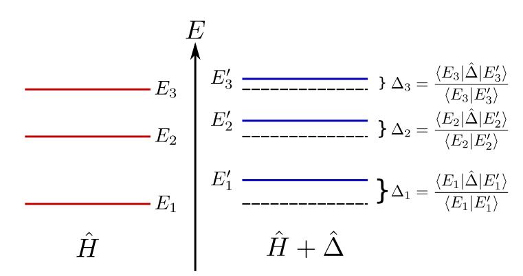
Conclusion: Measurable energy shifts caused by a perturbation are always (purely real) weak values.

JD, PRA 91 032116 (2015)

Role 4 : Weak Values as mean-field parameters

In reduced state dynamics, weak values appear as the correct estimations of parameters for the ensemble-averaged degrees of freedom.

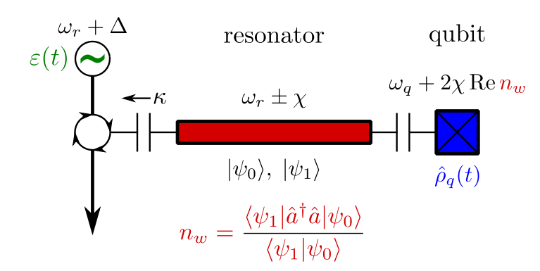
Circuit QED Example

\displaystyle \hat{H} = \frac{\omega_q}{2}\hat{\sigma}_z + \omega_r \hat{a}^\dagger \hat{a} + \chi \hat{\sigma}_z \hat{a}^\dagger \hat{a}

\displaystyle \hat{H} = \frac{\omega_q}{2}\hat{\sigma}_z + \omega_r \hat{a}^\dagger \hat{a} + \chi \hat{\sigma}_z \hat{a}^\dagger \hat{a}

At steady state, the balance of pump and decay from the resonator leaves the qubit entangled with distinct coherent states in the resonator:

Dispersive Coupling Hamiltonian:

|\Psi\rangle = c_0(t) |0\rangle |\psi_0\rangle + c_1(t) |1\rangle |\psi_1\rangle

This reduced state qubit coherence evolves as:

\rho_{01}(t) = c_1^*(t) c_0(t) \langle \psi_1(t) | \psi_0(t)\rangle

\rho_{01}(t) = c_1^*(t) c_0(t) \langle \psi_1(t) | \psi_0(t)\rangle

The coherence of the reduced qubit state is thus given by:

\partial_t \rho_{01}(t) = i[\omega_q + 2\chi \,n_w]\rho_{01}(t)

\partial_t \rho_{01}(t) = i[\omega_q + 2\chi \,n_w]\rho_{01}(t)

\displaystyle n_w \approx \frac{4\epsilon^2}{\kappa^2}\left[1 + i\frac{4\chi}{\kappa}\right] \equiv \bar{n} + i\frac{4\chi \bar{n}}{\kappa}

\displaystyle n_w \approx \frac{4\epsilon^2}{\kappa^2}\left[1 + i\frac{4\chi}{\kappa}\right] \equiv \bar{n} + i\frac{4\chi \bar{n}}{\kappa}

Photon number weak value!

Real part : AC Stark shift
Imaginary part : ensemble dephasing

\Delta\omega_q = 2\chi\,\text{Re}n_w = 2\chi\bar{n}

\Delta\omega_q = 2\chi\,\text{Re}n_w = 2\chi\bar{n}

\displaystyle \Gamma = 2\chi \,\text{Im}n_w = \frac{8\chi^2\bar{n}}{\kappa}

\displaystyle \Gamma = 2\chi \,\text{Im}n_w = \frac{8\chi^2\bar{n}}{\kappa}

JD, PRA 91 032116 (2015)

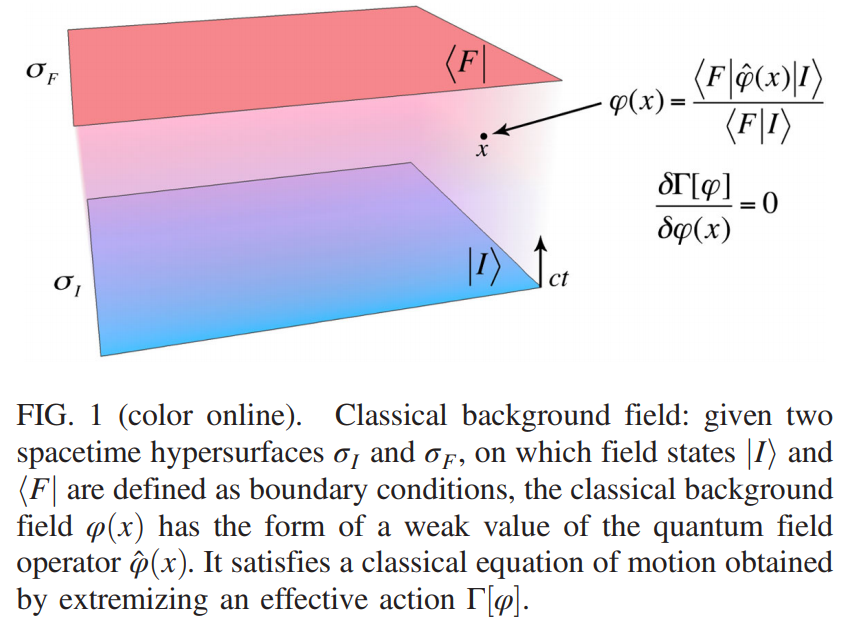
Field Theory Example

The usual field-theory prescription for finding the "classical" background field that describes the averaged configuration of the field is precisely a weak value.

Z[J] = {}_J\langle F| I \rangle_J = e^{iW[J]/\hbar}

Z[J] = {}_J\langle F| I \rangle_J = e^{iW[J]/\hbar}

\delta \hat{S} = \int d^4 x\, J(x) \hat{\varphi}(x)

\delta \hat{S} = \int d^4 x\, J(x) \hat{\varphi}(x)

\delta \langle F | I \rangle = \frac{i}{\hbar}\langle F | \delta \hat{S} | I \rangle

\delta \langle F | I \rangle = \frac{i}{\hbar}\langle F | \delta \hat{S} | I \rangle

Schwinger Variational Principle:

Probing Perturbation J(x):

Generating Functionals:

\varphi(x) \equiv \frac{\delta W[J]}{\delta J(x)} = \frac{\langle F | \hat{\varphi}(x)| I\rangle}{\langle F | I \rangle}

\varphi(x) \equiv \frac{\delta W[J]}{\delta J(x)} = \frac{\langle F | \hat{\varphi}(x)| I\rangle}{\langle F | I \rangle}

Classical Background Field:

JD et al., PRL 112 110407 (2014)

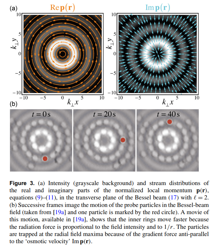
Example : Classical field Bessel beam

The connection to classical field clarifies why weak values appear as physical properties of a classical field, even when there is not an obvious "weak measurement" at the level of individual quanta of the field.

\displaystyle \text{Re}\,\mathbf{p}(\mathbf{r}) = \text{Re} \frac{\langle x | \hat{p} | \psi \rangle}{\langle x | \psi \rangle} = \frac{\omega}{c^2} \frac{S_o(\textbf{r})}{W(\textbf{r})}

\displaystyle \text{Re}\,\mathbf{p}(\mathbf{r}) = \text{Re} \frac{\langle x | \hat{p} | \psi \rangle}{\langle x | \psi \rangle} = \frac{\omega}{c^2} \frac{S_o(\textbf{r})}{W(\textbf{r})}

Orbital part of Poynting Vector

Energy density

Example : Momentum weak value appears as the local momentum of an optical field that can push probe particles around

Bliokh et al., NJP (2013) 10.1088/1367-2630/15/7/073022

Role 5 : Weak Values as a Classical Limit

Following the usual Hamilton-Jacobi approach to obtaining the quantum-to-classical transition, weak values appear as the correct classical correspondence.

\displaystyle i\hbar \partial_t |\psi(t)\rangle = \left[ \frac{\hat{p}^2}{2m} + V(\hat{x}) \right] |\psi(t)\rangle

\displaystyle i\hbar \partial_t |\psi(t)\rangle = \left[ \frac{\hat{p}^2}{2m} + V(\hat{x}) \right] |\psi(t)\rangle

Schrodinger Equation:

Define Hamilton's Principle Function :

S(t, x) \equiv -i\hbar \ln\langle x | \psi(t) \rangle

S(t, x) \equiv -i\hbar \ln\langle x | \psi(t) \rangle

\displaystyle p(t,x) \equiv \partial_x S(t,x) = \frac{-i\hbar\partial_x\psi(t,x)}{\psi(t,x)} = \frac{\langle x | \hat{p} | \psi(t) \rangle}{\langle x | \psi(t) \rangle}

\displaystyle p(t,x) \equiv \partial_x S(t,x) = \frac{-i\hbar\partial_x\psi(t,x)}{\psi(t,x)} = \frac{\langle x | \hat{p} | \psi(t) \rangle}{\langle x | \psi(t) \rangle}

Momentum defined in the usual way produces weak value of momentum operator:

Schrodinger's Equation can be written exactly as a Hamilton-Jacobi Equation:

\partial_t S(t, x) + H[t,x, p(t,x)] = 0

\partial_t S(t, x) + H[t,x, p(t,x)] = 0

\displaystyle \text{Re} H[t,x, p(t,x)] = \text{Re} \frac{\langle x | \hat{p}^2/2m + V(\hat{x}) | \psi \rangle}{\langle x | \psi \rangle} = \frac{(\text{Re}\,p(t,x))^2}{2m} + V(x) + Q(x)

\displaystyle \text{Re} H[t,x, p(t,x)] = \text{Re} \frac{\langle x | \hat{p}^2/2m + V(\hat{x}) | \psi \rangle}{\langle x | \psi \rangle} = \frac{(\text{Re}\,p(t,x))^2}{2m} + V(x) + Q(x)

Imaginary part is a continuity equation for probability. Real part is classical HJ Equation.

\displaystyle Q(x) = \frac{\langle x| (\hat{p} - \text{Re}p(t,x))^2 | \psi(t) \rangle}{\langle x | \psi(t) \rangle}

\displaystyle Q(x) = \frac{\langle x| (\hat{p} - \text{Re}p(t,x))^2 | \psi(t) \rangle}{\langle x | \psi(t) \rangle}

Quantum Correction: "Weak Variance" of momentum away from weak value

Correction vanishes in usual limit for ray optics (wavelength small). The correct classical momentum is a weak value.

Conclusions

Weak values play many roles in the quantum formalism:

Conditioned average of weakly measured observable
Multiplicative corrections to amplitudes from interactions
Minimum error estimations of observables
Spectral shifts due to perturbations
Classical mean field properties
Classical limit for observable values

Thank you!

z_s

z_s