Weak values

From superoscillations to mean-field estimates

Justin Dressel
Institute for Quantum Studies, Chapman University

Superoscillations Conference, 6/15/2019

Weak Value:

A "conditioned expectation value" that appears naturally in quantum dynamics

\displaystyle A_w \equiv \frac{\langle \phi | \hat{A} | \psi \rangle}{\langle \phi | \psi \rangle}

It is conditioned in the sense that a complete expectation value can be partitioned into a convex mixture of weak values, each specific to a particular "postselection".

\displaystyle \langle A \rangle \equiv \langle \psi | \hat{A} | \psi \rangle = \sum_n \langle \psi | \phi_n \rangle\langle \phi_n |\hat{A} | \psi \rangle = \sum_n |\langle \phi_n | \psi \rangle|^2 \frac{\langle \phi_n | \hat{A} | \psi \rangle}{\langle \phi_n | \psi \rangle} = \sum_n P_n\, A_{w,n}

Weak values are not constrained by the spectra of the operator A due to quantum interference between pre- and post-selections.

Superoscillations in that interference cause anomalous values.

\hat{H}|E_k\rangle = E_k |E_k \rangle

(\hat{H}+\hat{\Delta})|E'_j\rangle = E'_j |E'_j \rangle

\langle E'_j |(\hat{H}+\hat{\Delta})|E_k\rangle = E'_j \langle E'_j | E_k \rangle = E_k \langle E'_j | E_k \rangle + \langle E'_j |\hat{\Delta}| E_k \rangle

\displaystyle E'_j - E_k = \frac{\langle E'_j | \hat{\Delta} | E_k \rangle}{\langle E'_j | E_k \rangle}

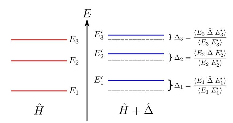
Measurable energy shifts caused by a perturbation are always (purely real) weak values.

This means that strange values outside the spectrum of the perturbation are measurable.

JD, PRA 91 032116 (2015)

Example: When a perturbation is added to a system, its energy spectra will shift by weak values of the perturbation.

\hat{Z} = |1\rangle\langle 1 | - |0\rangle\langle 0|

|\psi \rangle = |1\rangle

\langle f | = \langle 0 |

\displaystyle \hat{H} = \frac{\omega}{2} \left( |1\rangle\langle 0| + |0\rangle\langle 1|\right)

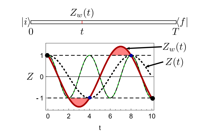
Simple Example: Time-dependent weak value

Whenever the observable is an eigenvalue with certainty, the weak value must match.

If the evolution is not consistent with the boundary conditions, then the weak value smoothly interpolates while preserving both the certainty of the eigenvalues and the periodicity of the evolution.

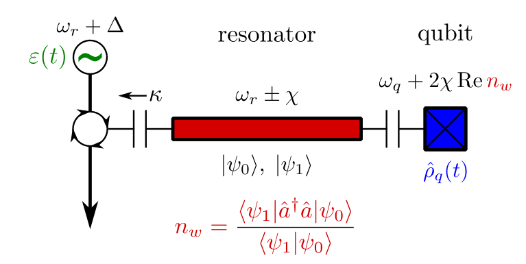
Nontrivial Example: Circuit QED

\displaystyle \hat{H} = \frac{\omega_q}{2}\hat{\sigma}_z + \omega_r \hat{a}^\dagger \hat{a} + \chi \hat{\sigma}_z \hat{a}^\dagger \hat{a}

At steady state, the balance of pump and decay from the resonator leaves the qubit entangled with distinct coherent states in the resonator:

Dispersive Coupling Hamiltonian:

This reduced state qubit coherence evolves as:

\rho_{01}(t) = c_1^*(t) c_0(t) \langle \psi_1(t) | \psi_0(t)\rangle

The coherence of the reduced qubit state is thus given by:

\partial_t \rho_{01}(t) = i[\omega_q + 2\chi \,n_w]\rho_{01}(t)

\displaystyle n_w \approx \frac{4\epsilon^2}{\kappa^2}\left[1 + i\frac{4\chi}{\kappa}\right] \equiv \bar{n} + i\frac{4\chi \bar{n}}{\kappa}

Photon number weak value!

Real part : AC Stark shift
Imaginary part : ensemble dephasing

\Delta\omega_q = 2\chi\,\text{Re}n_w = 2\chi\bar{n}

\displaystyle \Gamma = 2\chi \,\text{Im}n_w = \frac{8\chi^2\bar{n}}{\kappa}

JD, PRA 91 032116 (2015)

\mathcal{D}_\psi (\hat{A},\hat{B}) = \langle\psi |(\hat{A} - \hat{B})^2 |\psi\rangle

Consider a distance measure between two observables (mean-squared "operator error"):

Suppose you wish to estimate \(\hat{A}\), but measure a basis \(\{|f\rangle\}\) that is not its eigenbasis. What is the closest observable to \(\hat{A}\) that you can estimate? That is, what values \(\bar{a}_f\) should you assign to each observed outcome to minimize the operator error?

\hat{A}_{\text{est}} = \sum_f \bar{a}_f |f\rangle\langle f|

\mathcal{D}_\psi(\hat{A},\hat{A}_{\text{est}}) = \langle \psi | \hat{A}^2 | \psi\rangle - \sum_f |\langle f | \psi \rangle |^2 \left[\text{Re}\frac{\langle f | \hat{A} | \psi \rangle}{\langle f | \psi \rangle}\right]^2 + \sum_f |\langle f | \psi \rangle | ^2 \left[ \bar{a}_f - \text{Re}\frac{\langle f | \hat{A} | \psi\rangle}{\langle f | \psi \rangle}\right]^2

Only dependence on estimated values

Conclusion: the real part of the weak value is the best estimate for an observable value given the known boundary conditions

\bar{a}_f = \text{Re}\frac{\langle f | \hat{A} | \psi \rangle}{\langle f | \psi \rangle}

Partial explanation: Weak values as best estimates

\hat{U}_g = e^{-ig\hat{A}}

\displaystyle \langle \phi | \hat{U}_g|\psi\rangle = \frac{\langle \phi | e^{-ig\hat{A}}|\psi\rangle}{\langle \phi | \psi \rangle} \langle \phi | \psi \rangle = \left[\sum_{n=0}^\infty (-ig)^n A_w^{(n)}\right] \langle \phi | \psi \rangle

|\psi\rangle

\langle\phi |

Prepare

Transform

Measure

\displaystyle A_w^{(n)} \equiv \frac{\langle \phi | \hat{A}^n | \psi \rangle}{\langle \phi | \psi \rangle}

"Modular Value"

Multiplicative amplitude correction from transformation

nth order "Weak Value"

Amplitude

Weak values in evolution amplitudes

When g is sufficiently small, the 1st order weak value dominates the amplitude

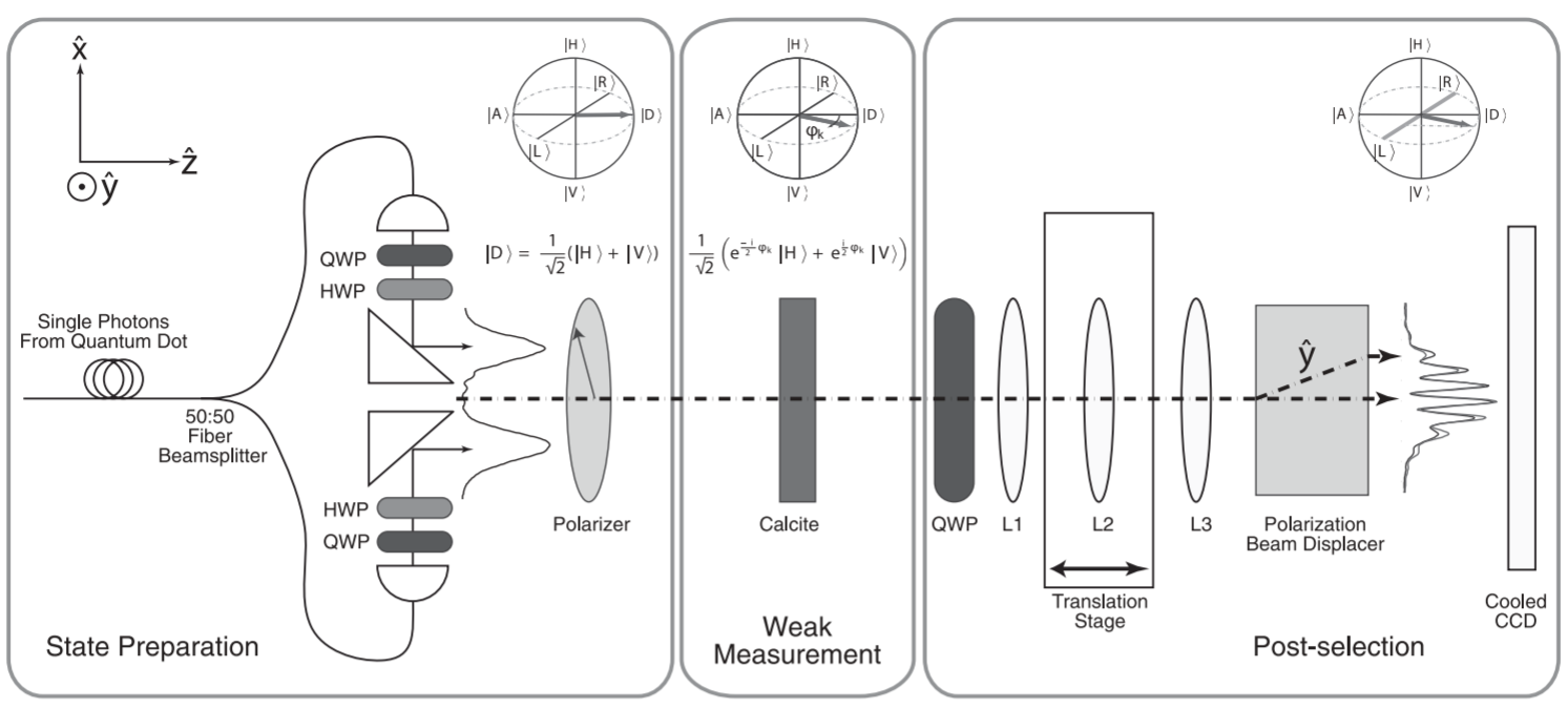
Example: Sagnac Beam-tilt Experiment

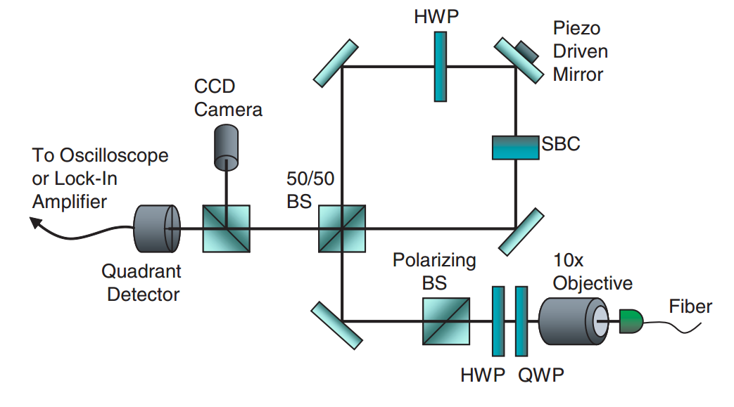
Howell lab, Rochester

PRL 102, 173601 (2009)

Ultra-sensitive to beam deflection: ~560 femto-radians of tilt detected

\phi\;\text{(phase offset)}

k\;\text{(tilt)}

x\;\text{(signal)}

\sigma\;\text{(beam waist)}

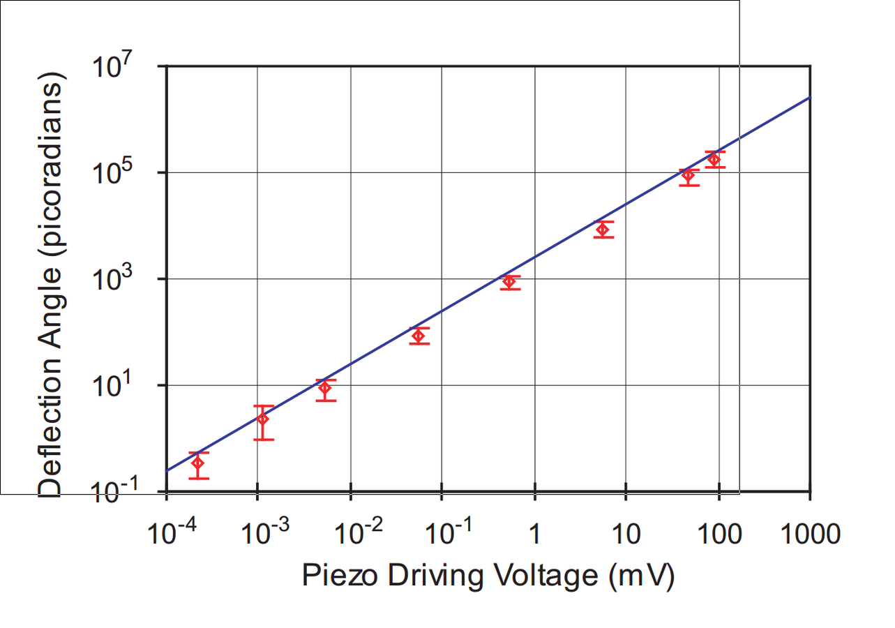
Weak Value Analysis

|i\rangle \propto i|\!\circlearrowleft\rangle + |\!\circlearrowright\rangle

|f\rangle \propto e^{i\phi/2}|\!\circlearrowleft\rangle - ie^{-i\phi/2}|\!\circlearrowright\rangle

|\psi, i\rangle \to \langle p, f | \exp(-i k \hat{x}\hat{W}) | \psi, i \rangle \approx \langle f | i \rangle \langle p - k W_w | \psi \rangle

\hat{W} = |\!\circlearrowleft\rangle\langle\!\circlearrowleft | - |\!\circlearrowright\rangle\langle\!\circlearrowright |

W_w = \frac{\langle f |\hat{W}|i\rangle}{\langle f | i \rangle} = i\cot\frac{\phi}{2} \approx \frac{2i}{\phi}

\phi\;\text{(phase offset)}

k\;\text{(tilt)}

x\;\text{(signal)}

\sigma\;\text{(beam waist)}

Angular tilt (transverse momentum) amplified by large weak value.

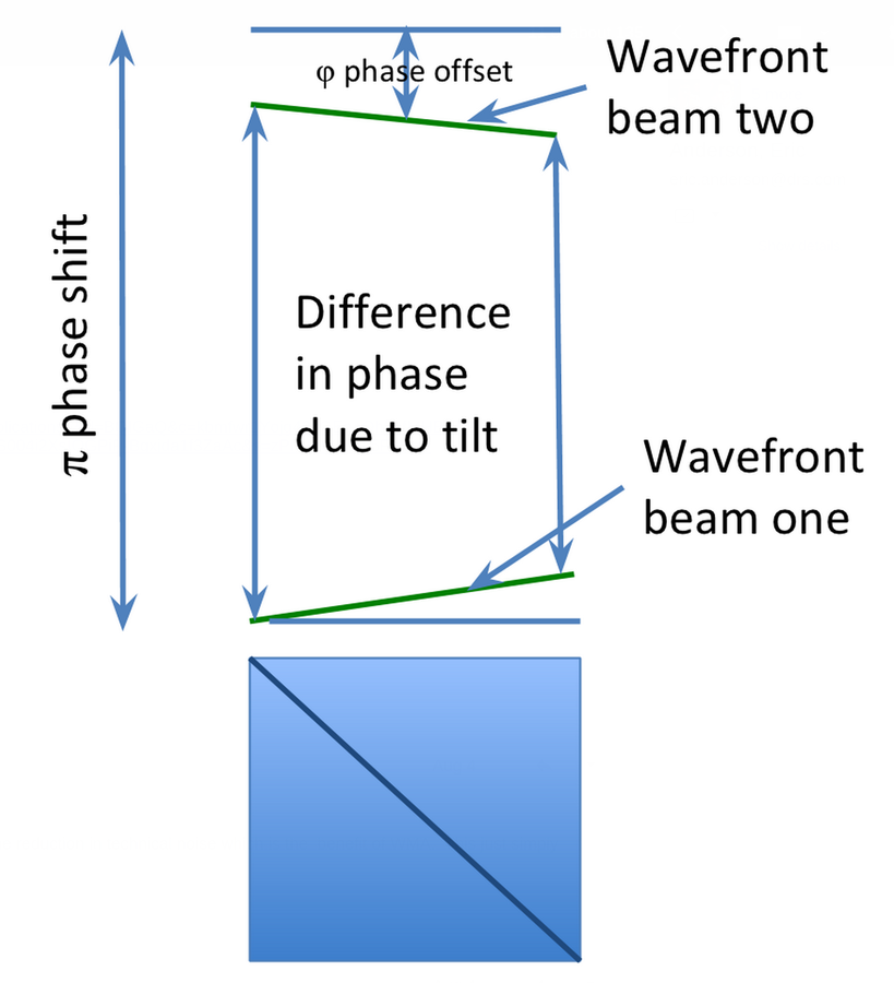
Collimated Beam Analysis

|i\rangle = \frac{i|\!\circlearrowleft\rangle + |\!\circlearrowright\rangle}{\sqrt{2}}

|f\rangle = \frac{e^{i\phi/2}|\!\circlearrowleft\rangle - ie^{-i\phi/2}|\!\circlearrowright\rangle}{\sqrt{2}}

|\psi, i\rangle \to \langle x, f | \exp(-i k \hat{x}\hat{W}) | \psi, i \rangle = \langle x|\hat{M}_f\,|\psi\rangle = i\sin(\phi/2 - kx)\langle x | \psi\rangle

\hat{W} = |\!\circlearrowleft\rangle\langle\!\circlearrowleft\! | - |\!\circlearrowright\rangle\langle\!\circlearrowright\! |

\phi\;\text{(phase offset)}

k\;\text{(tilt)}

x\;\text{(signal)}

\sigma\;\text{(beam waist)}

\hat{M}_f = \langle f | \exp(-i k \hat{x}\hat{W}) | i \rangle = i \sin(\phi/2 - k\hat{x})

P(x) = |\langle x,f| \psi,i\rangle|^2 = \sin^2(\phi/2 - kx)\,P_0(x) = \frac{\sin^2(\phi/2 - kx)}{\sqrt{2\pi\sigma^2}} e^{-(x/\sigma)^2/2}

Original profile of beam becomes modulated by postselection interference.

JD et al., PRA 88 , 023801 (2013)

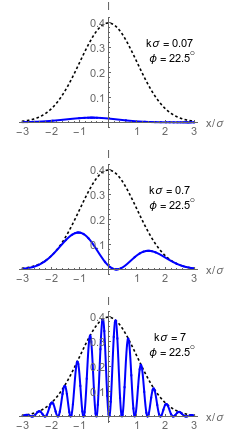
Collimated Dark Port Profiles

Left: Wavefront tilt mechanism producing spatial modulation

Right: Asymmetric dark port profiles in different regimes

Dashed envelope: input beam intensity

Solid curve:

dark port intensity

Top right:

weak value regime

Middle right:

double lobe regime

Bottom right:

misaligned regime

k\sigma \ll \phi \ll 1

\phi\ll k\sigma \ll 1

\phi\ll 1 \ll k\sigma

Weak value regime

k\sigma \ll \phi \ll 1

Dark port has single lobe that approximates a displaced Gaussian centered at:

\langle x/\sigma \rangle \propto (\mathbf{k}/\phi)\sigma

Tiny beam deflections can be distinguished, but with low output intensity.

I \propto \phi^2

\displaystyle i\hbar \partial_t |\psi(t)\rangle = \left[ \frac{\hat{p}^2}{2m} + V(\hat{x}) \right] |\psi(t)\rangle

Schrodinger Equation:

Define Hamilton's Principle Function :

S(t, x) \equiv -i\hbar \ln\langle x | \psi(t) \rangle

\displaystyle p(t,x) \equiv \partial_x S(t,x) = \frac{-i\hbar\partial_x\psi(t,x)}{\psi(t,x)} = \frac{\langle x | \hat{p} | \psi(t) \rangle}{\langle x | \psi(t) \rangle}

Momentum defined in the usual way produces weak value of momentum operator:

Schrodinger's Equation can be written exactly as a Hamilton-Jacobi Equation:

\partial_t S(t, x) + H[t,x, p(t,x)] = 0

\displaystyle \text{Re} H[t,x, p(t,x)] = \text{Re} \frac{\langle x | \hat{p}^2/2m + V(\hat{x}) | \psi \rangle}{\langle x | \psi \rangle} = \frac{(\text{Re}\,p(t,x))^2}{2m} + V(x) + Q(x)

Imaginary part is a continuity equation for probability. Real part is classical HJ Equation.

\displaystyle Q(x) = \frac{\langle x| (\hat{p} - \text{Re}p(t,x))^2 | \psi(t) \rangle}{\langle x | \psi(t) \rangle}

Quantum Correction: "Weak Variance" of momentum away from weak value

Correction vanishes in usual limit for ray optics (wavelength small). The correct classical momentum is a weak value.

Weak values in classical correspondence

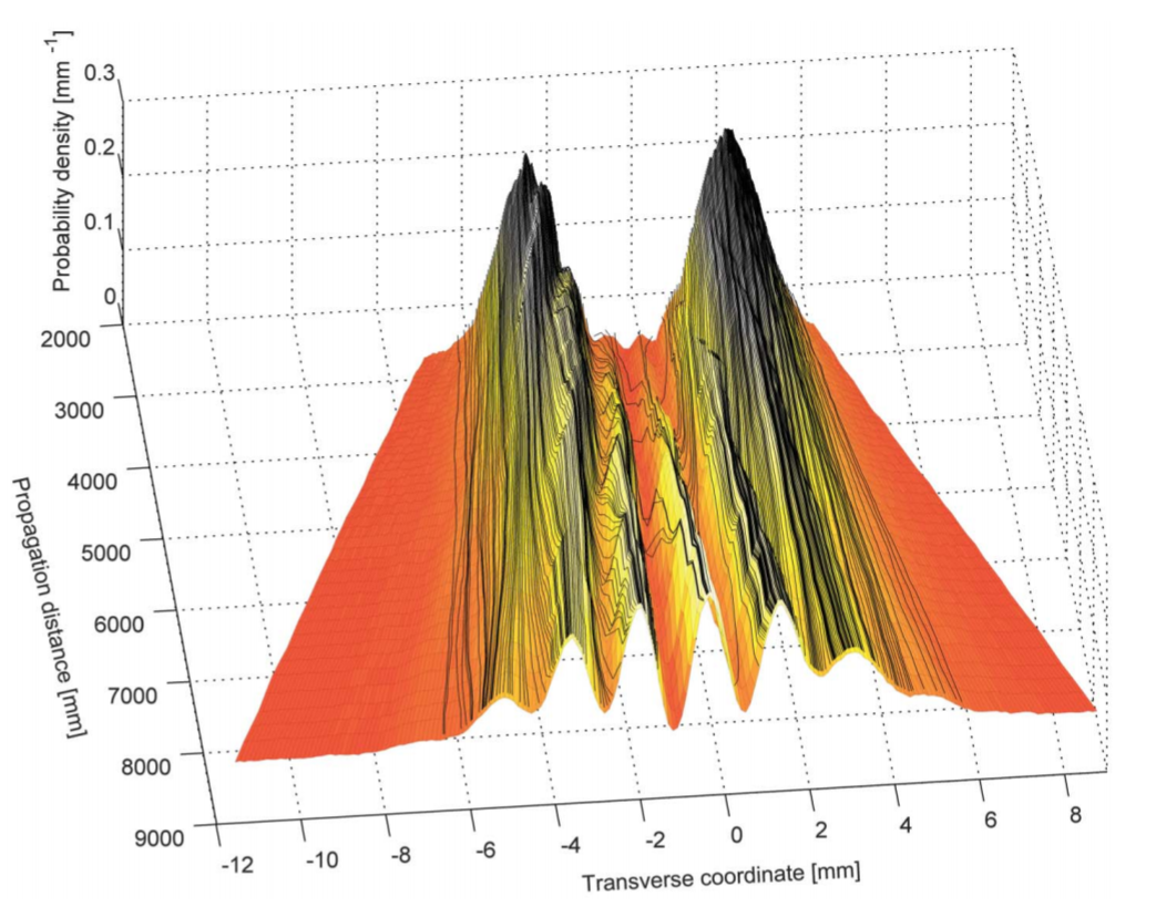
Example : Classical field trajectories

Weak values also appear as physical properties of a classical field, even when there is not an obvious "weak measurement" at the level of individual field quanta.

\displaystyle \text{Re}\,\mathbf{p}(\mathbf{r}) = \text{Re} \frac{\langle x | \hat{p} | \psi \rangle}{\langle x | \psi \rangle} = p_B(x)

Local (Bohmian) momentum average

Example : Momentum weak value appears as the local momentum of an optical field. This can be measured and used to reconstruct "averaged trajectories" for how light passes through a double-slit to produce wave interference.

The average local momentum corresponds to the local optical pressure felt by small probe particles.

Kocsis et al., Science 332, 1170 (2011)

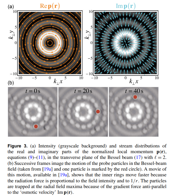
Example : Classical field Bessel beam

Both real and imaginary parts of this local momentum average also describe physical properties of classical "vortex beams" like Bessel beams.

\displaystyle \text{Re}\,\mathbf{p}(\mathbf{r}) = \text{Re} \frac{\langle x | \hat{p} | \psi \rangle}{\langle x | \psi \rangle} = \frac{\omega}{c^2} \frac{S_o(\textbf{r})}{W(\textbf{r})}

Orbital part of Poynting Vector

Energy density

The real part of the momentum weak value appears as the circulating local momentum that can push probe particles around.

The imaginary part appears as the radial confining momentum that sculpts the optical profile into rings.

Bliokh et al., NJP (2013) 10.1088/1367-2630/15/7/073022

Weak values best describe the average of the noisy voltage signal obtained while measuring quantum state trajectories

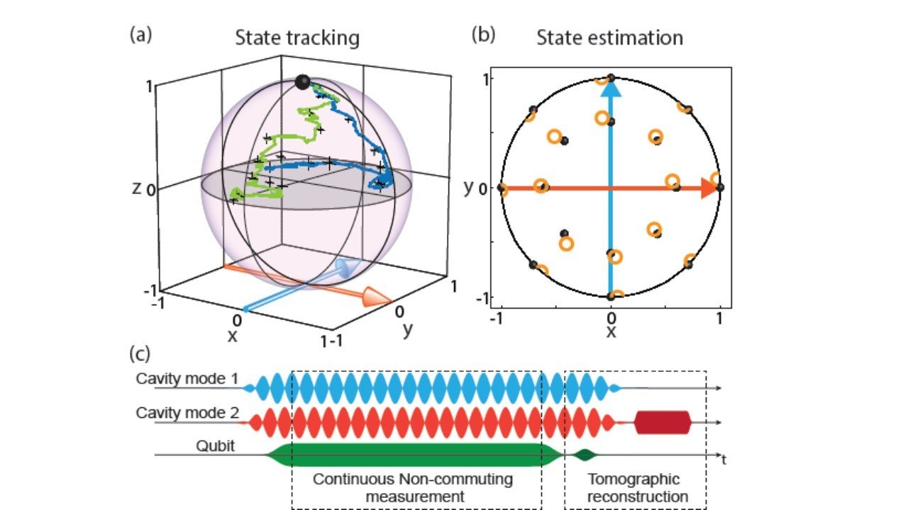
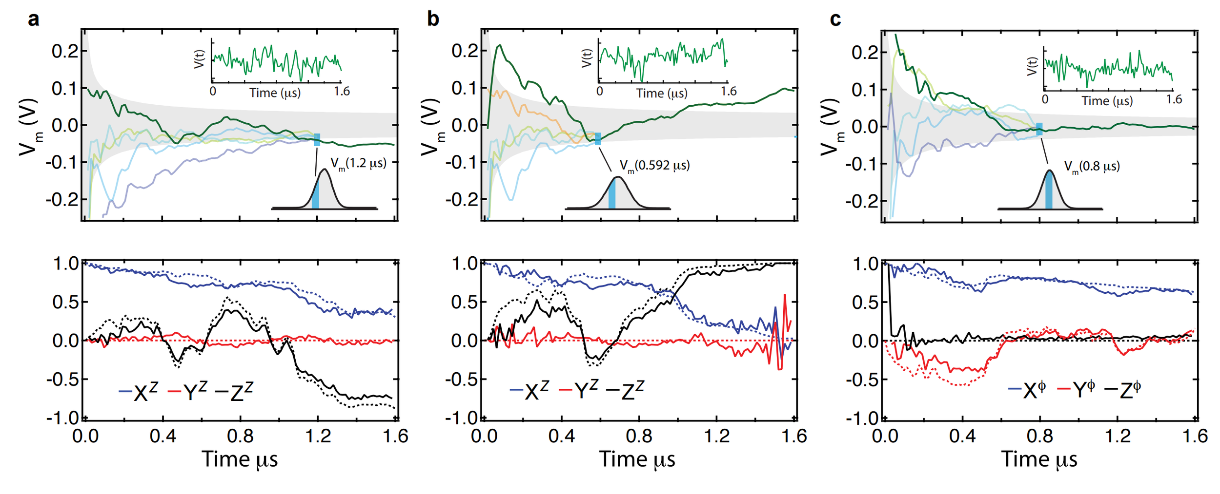
Weak values in time-continuous monitoring

Murch et al., Nature 502, 211 (2013)

Hacohen-Gourgy et al., Nature 538, 491 (2016)

Signal filtering example: Simultaneous X + Z

Simple single pole filter

Simultaneous (here X+Z) measurements work well

(with stronger measurements)

One can track multiple observables simultaneously for a single trajectory with reasonable (~90%) fidelity, without a master equation

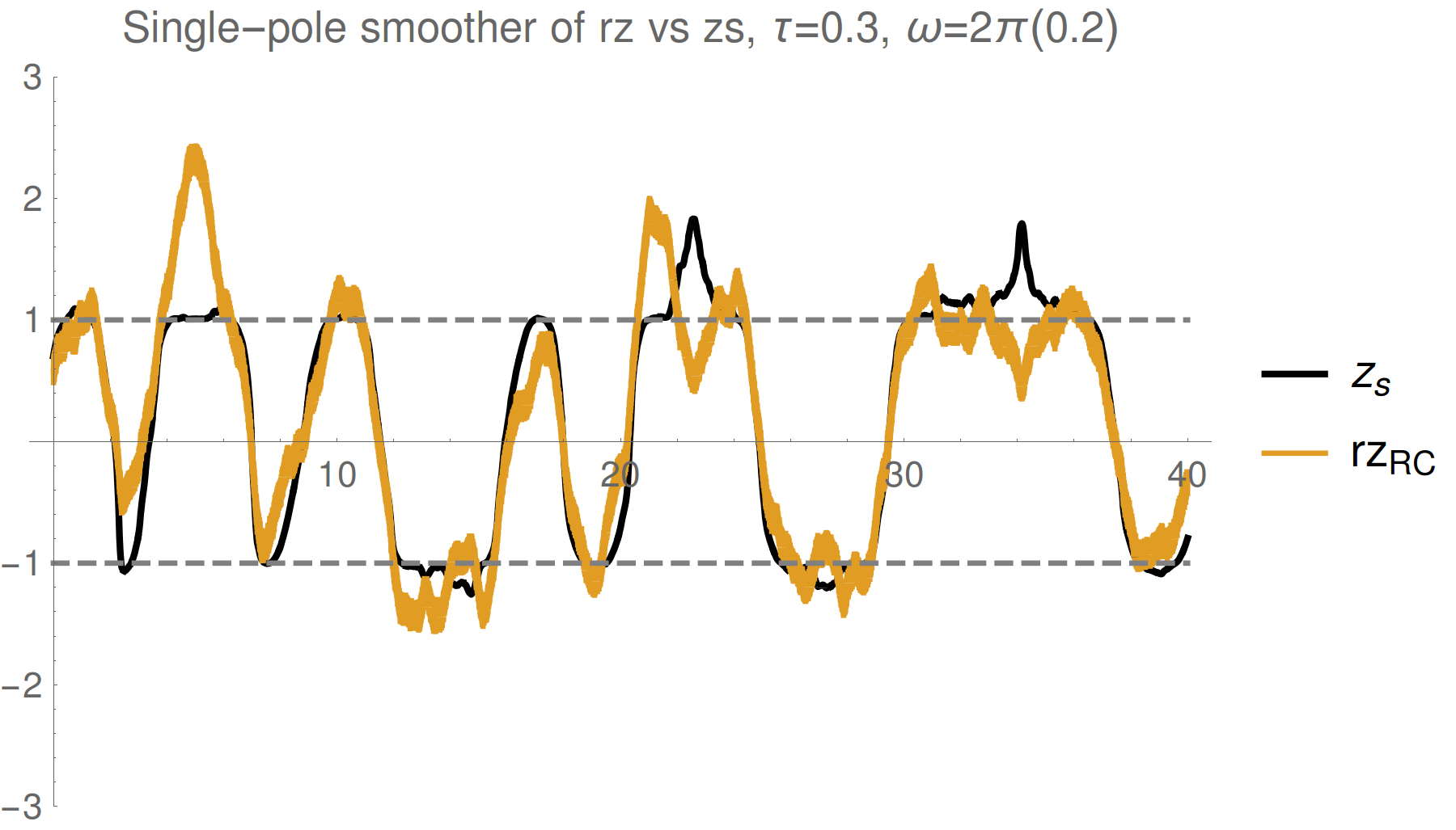
Filtering works, but doesn't quite follow expectation values - what does it follow?

see also Ruskov et al. PRL 105 100506 (2010): >90% state fidelity with 3 axis monitoring + filtering

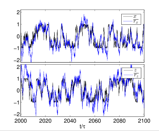
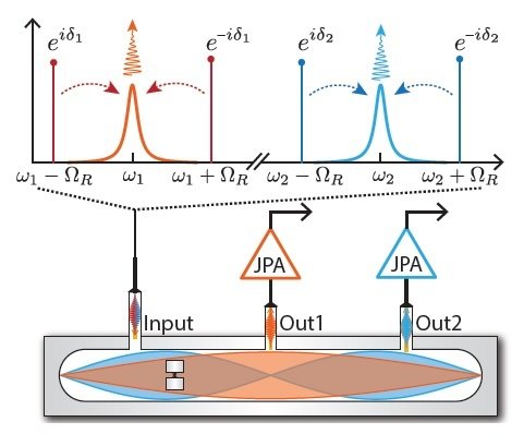
Hacohen-Gourgy et al., Nature 538, 491 (2016)

Consider a single collected readout r(t), but omit one point at t=t1.

What distribution P[r(t1)] describes the likelihood of the omitted point?

Past Readout Distribution

P(r\, |\, \vec{r}_{\mathrm{past}},\, \vec{r}_{\mathrm{future}}) = \frac{P(r,\, \vec{r}_{\mathrm{future}}\,|\,\vec{r}_{\mathrm{past}})}{\sum_r P(r,\, \vec{r}_{\mathrm{future}}\,|\,\vec{r}_{\mathrm{past}})} \approx \frac{\exp\left[-\frac{dt}{2\tau}(r-z_s)^2\right]}{\sqrt{2\pi\tau/dt}}

Discretize time into bins of size dt - assume Markovian Gaussian measurements:

We recover approximate Gaussian noise, as expected:

r(t) = z_s(t) + \sqrt{\tau}\,\xi(t)

The collected readout follows a shifted mean value

(Consequence of the measurement backaction producing non-Markovian correlations)

The mean is the expectation value of Z only on the boundary, with unknown future record (as appropriate for simulation)

In between boundaries, it is a conditioned (smoothed) estimate

Smoothed Observable Estimate

r(t) = z_s(t) + \sqrt{\tau}\,\xi(t)

Optimally filtering/smoothing a single collected readout

will remove the Gaussian noise, and recover the

shifted observable value, not the expectation value

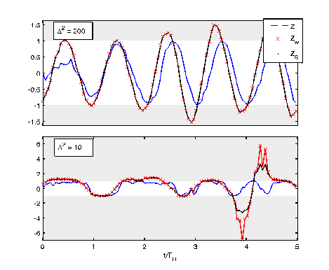
z_s = z_w\, \left[\frac{2}{(1+e^{-dt/2\tau}) + z_c\,(1-e^{-dt/2\tau})}\right] \approx z_w

Weak regime

Strong regime

\displaystyle z_w = \mathrm{Re}\frac{\mathrm{Tr}[E_{\vec{r}_{\mathrm{future}}}\,Z\,\rho_{\vec{r}_{\mathrm{past}}}]}{\mathrm{Tr}[E_{\vec{r}_{\mathrm{future}}}\,\rho_{\vec{r}_{\mathrm{past}}}]}

Smoothed (shifted) observable mean:

Depends on a weak value and a quadratric correction:

\displaystyle z_c = \frac{\mathrm{Tr}[E_{\vec{r}_{\mathrm{future}}}\,Z\,\rho_{\vec{r}_{\mathrm{past}}}\,Z]}{\mathrm{Tr}[E_{\vec{r}_{\mathrm{future}}}\,\rho_{\vec{r}_{\mathrm{past}}}]}

\rho_{\vec{r}_{\mathrm{past}}} = \mathcal{M}_{\vec{r}_{\mathrm{past}}}[\rho_0]

E_{\vec{r}_{\mathrm{future}}} = \mathcal{M}^*_{\vec{r}_{\mathrm{future}}}[1]

Non-Markovian dependence on both

past state and future effect matrix:

Consistent with:

Aharonov PRL 60, 1351 (1988), Wiseman PRA 65, 032111 (2002), Tsang PRL 102, 250403 (2009), Dressel PRL 104, 240401 (2010), Dressel PRA 88, 022107 (2013), Mølmer PRL 111, 160401 (2013)

( No additional ad hoc postselection)

Hypothesis Test from Readout

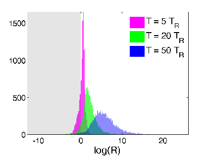
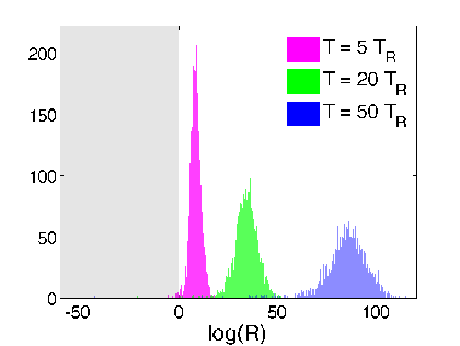
Verification: Look at relative log-likelihood of
generating the raw readout from adding Gaussian noise to the two estimates - equivalent to a hypothesis test

\displaystyle \log(R) \equiv \log\frac{P(r|z)}{P(r|z_s)}

Discriminator:
(>0 implies smoothed value more likely than expectation value to generate readout)

T_R : \mathrm{Rabi\, period}

\Delta^2 : \tau_z/dt

Strong regime

Weak regime

T : \mathrm{traj.\,length}

smoothed better

Yes. The smoothed value is objectively more likely to generate the observed readout from additive noise

z_s

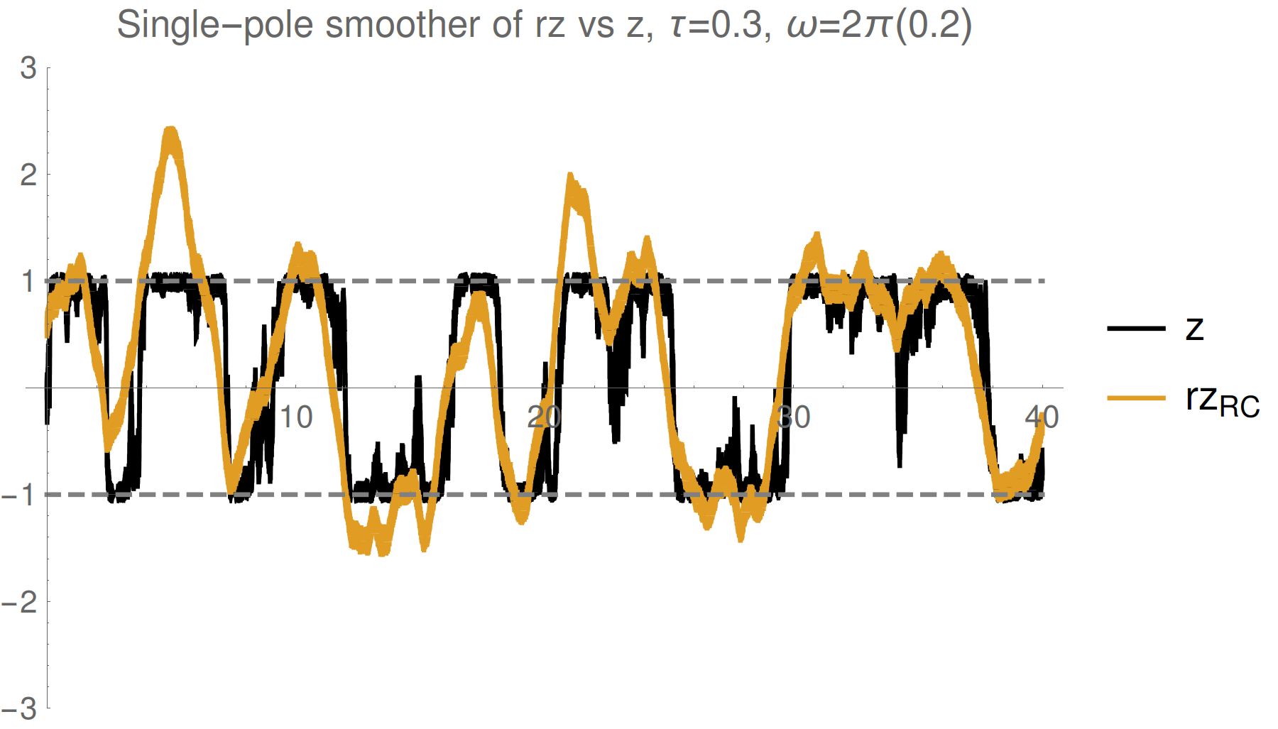
Is this really true? The estimate is a weak value that can exceed eigenvalue range

Corroboration by Third Party

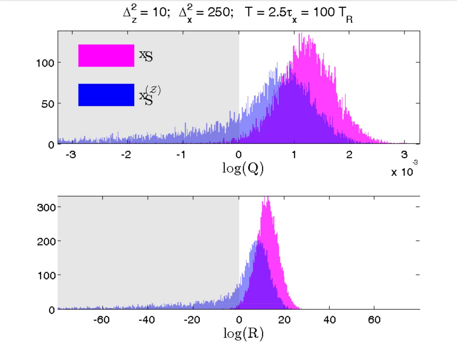
Variation: Suppose Bob is weakly monitoring a different observable (X) at the same time

If Alice is more strongly monitoring (Z) and has no access to Bob's record, does her smoothed estimate of X (not measured by her) still correspond to Bob's record?

Yes. Even without access to Bob's record, Alice can construct a smoothed estimate from her record that fits Bob's observed record better than the expectation value (computed either from Alice's subjective state or the most pure state with perfect knowledge of both records)

Test verifies that a better model of the relevant dynamics produces an objectively closer fit to the collected record

Smoothed estimate is operationally meaningful

RMS Error Test

Hypothesis Test

Blue : Alice does not know Bob's record

Pink : Alice knows both records

smoothed better

[Similar question to Guevara, Wiseman PRL 115, 180407 (2015) ]

Conclusions

The superoscillations intrinsic to weak values play many roles in the quantum formalism:

Conditioned average of weakly measured observable
Spectral shifts due to perturbations
Classical mean field properties
Classical limit for observable values
Multiplicative corrections to amplitudes from interactions
Minimum error estimations of observables
Many more applications to come!

Thank you!

z_s