ON THE INTERPLAY BETWEEN MICROKINETICS
AND
TURBULENCE IN SPACE PLASMAS
Ramiz A. Qudsi
Dept. of Phys. and Astronomy, University of Delaware, DE
21 June, 2021
ahmadr@udel.edu
Advisor: Bennett A. Maruca
In this talk
- Plasma and why it is important to study.
- Different kinds of plasmas
- How we study them
- Instabilities in a plasma
- Intermittency in plasmas
- Origin
- Measuring it
- Consequence
- Interplay between linear and nonlinear process
- Magnetic field topology reconstruction
- Conclusion
https://slides.com/qudsi/thesis/
Plasma
- Ionosphere
- Terrestrial Magnetosheath
- Solar wind
- At 1 au
- Inner Heliosphere (0.2 au)
- Outer Heliosphere
- Interstellar Medium (ISM)
- Intergalactic Medium (IGM)
99.9% of the observable universe is in plasma state
Simulations
- PIC
- MHD
- Hybrid
Experiment/Lab Plasmas
Space Plasmas
https://news.engin.umich.edu/2018/08/the-end-of-the-mission/
- It is the fourth state of matter.
- Consists of charged particles and is generally neutral.

https://en.wikipedia.org/wiki/Magnetosphere
Interaction between Solar Wind and Earth's Magnetic Field
1) Bow shock.
2) Magnetosheath.
3) Magnetopause.
4) Magnetosphere.
5) Northern tail lobe.
6) Southern tail lobe.
7) Plasmasphere.
Typical Values
| 0.2 au | 1 au | Magnetosheath | |
|---|---|---|---|
| Magnetic Field | 70 | 5 | 20 |
| Ion-density | 150 | 5 | 30 |
| Ion-speed | 400 | 450 | 250 |
| Ion-temperature | 1 | 3 | 2.5 |
$$\rm{(cm^{-3})}$$
$$(\rm{nT})$$
$$\rm{(km/s)}$$
$$\rm{(10^6K)}$$
Studying Plasma
Vlasov Equation
Equation of Motion
Maxwell's Equation
Dispersion Relation
is the distribution function of plasma for species j
$$f_j$$
Linear Dispersion Equation
Vlasov Equation
Linearization
real
Maximum value of growth rate of a given mode for all k and directions
instability growth rate
imaginary
(Marsch, JGRL-1982)
VDF: Probability distribution function of phase space density
$$\hat{B}$$
Temperature Anisotropy:
Ratio of perpendicular and parallel temperatures
$$R_j = \frac{T_{\perp j}}{T_{\parallel j}}$$
Beta:
Ratio of thermal and magnetic pressure
$$\beta_{\parallel j} \equiv \frac{n_j\,k_{\rm B}\,T_{\parallel j}}{B^2\,/\,(2\,\mu_0)}$$
Solar Wind, 1 au
Magnetosheath


(Maruca, ApJ-2018)
Solar Wind, 1 au
Magnetosheath

(Hellinger, GRL-2006)

(Maruca, ApJ-2018)
Solar Wind, 1 au
Magnetosheath

(Qudsi, In-prep)

(Huang, ApJS-2020)
3-D PIC simulation
Solar Wind, 0.2-au
(Qudsi, ApJ-2020)
2.5-D PIC simulation
3-D PIC simulation
(Qudsi, ApJ-2020)
MMS Observation
(Qudsi, ApJ-2020)
Intermittency comparison between spacecraft observation and simulation
MMS
Wind
Measuring Intermittency
Intermittency: Burstiness
Distribution is not uniform and has localized structures
Measuring intermittency
(Greco, GRL-2008)
Lag in distance
Non-Gaussianity
: Time lag
(Osman, PRL-2012)
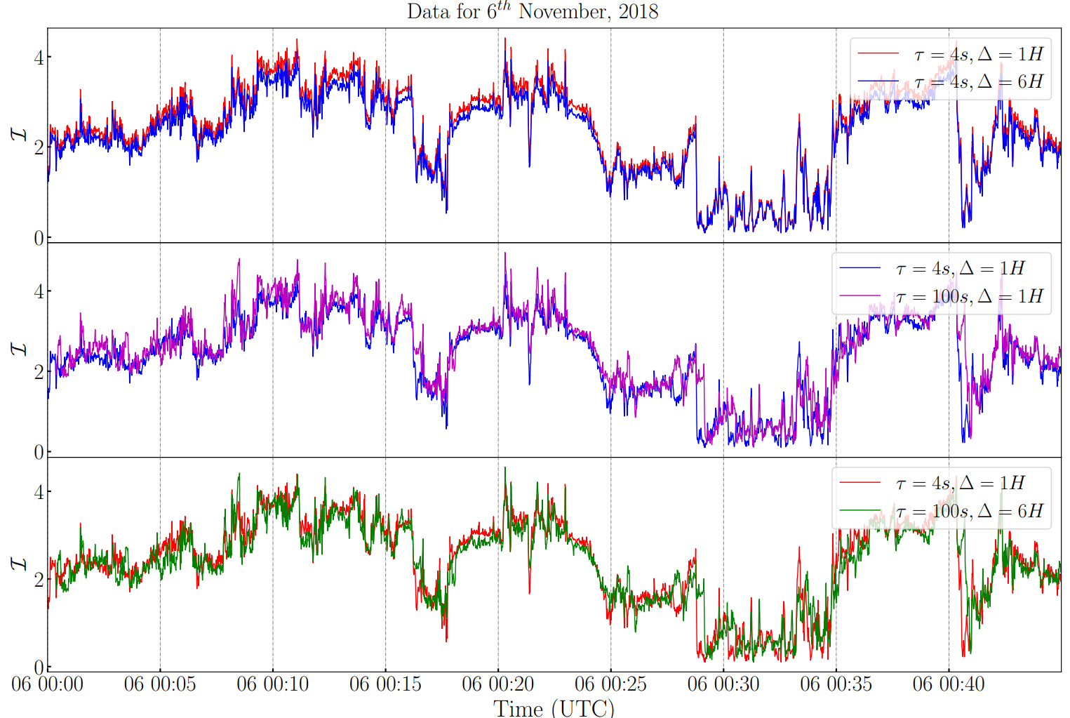
What value of and one should choose?
PVI
(Assuming Taylor hypothesis)
PSP : Encounter 1 (second half)
(Qudsi, ApJS-2020)
Conditional Temperature Averages
(Qudsi, ApJS-2020)
Non-linear Processes
Turbulence
- microinstability processes
- strongly nonlinear intermittent processes
Distortion of VDF
Microinstabilities
Intermittency
Turbulence
We estimate it from the spectral amplitude near the ion-inertial scale
Non-linear time scale
$$(\omega_{nl})$$
$$\omega_{\rm nl} \left(\vec{r}\right) \sim { \delta b_{\ell}}/{\ell}$$
$$\delta b_{\ell} = \left \lvert\hat{\boldsymbol{\ell}} {\cdot} \left[\vec{b} \left(\vec{r} + \vec{\ell}\right) - \vec{b} \left(\vec{r}\right)\right]\right\lvert$$
$$ b = \left\lvert \vec{B}/\vec{V_A}\right\lvert, \ell \sim 1/k_{\max}$$
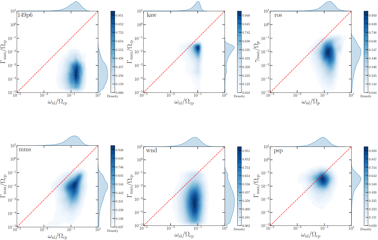
Comparison between and :
$$\omega_{\rm nl}$$
$$\Gamma_{\max}$$
Comparison between and
$$\omega_{\rm nl} \hspace{2em} \Gamma_{\max}$$
(Qudsi2021a, in prep)
MMS
Wind
Comparison between and
$$\omega_{\rm nl} \hspace{2em} \Gamma_{\max}$$
(Bandyopadhyay, PRL-2021,
under review)
Comparison between and
$$\omega_{\rm nl} \hspace{2em} \Gamma_{\max}$$
(Qudsi2021a, in prep)
Comparison between and
$$\omega_{\rm nl} \hspace{2em} \Gamma_{\max}$$

(Qudsi2021a, in prep)
Solar Wind, 1 au
(Maruca, ApJ-2018)
Solar Wind, 1 au
Magnetosheath
For any given system how do we figure out which one is most relevant?
A lot better understanding of turbulence cascade in plasmas
Complete 3D structure of interplanetary magnetic field
Comparison between and
$$\omega_{\rm nl} \hspace{2em} \Gamma_{\max}$$

(Qudsi2021a, in prep)
Magnetic Field Reconstruction
Gaussian Process Regression
It is a probabilistic data imputation method
$$m(\mathbf{x}) = \mathbb{E}[f(\mathbf{x})]$$
Mean function
$$k(\mathbf{x}, \mathbf{x'}) = \mathbb{E}[(f(\mathbf{x}) - m(\mathbf{x}))(f(\mathbf{x'}) - m(\mathbf{x'}))]$$
Covariance function
$$f(\mathbf{x}) \sim \mathcal{GP}\left(m(\mathbf{x}), k(\mathbf{x}, \mathbf{x'})\right)$$
Gaussian Processes


Constant
Linear
RBF
Matern
Kernels
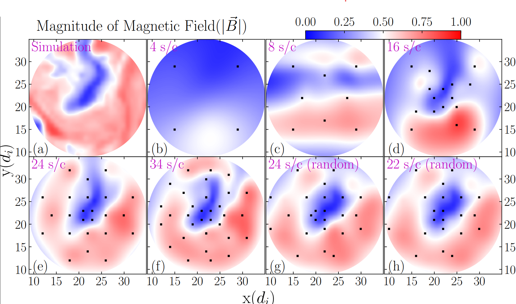
Reconstructed Magnetic Field
(Maruca, Frontiers-2021)
Reconstructed Magnetic Field

Conclusion:
- Linear instabilities are distributed intermittently as are coherent structures for all the cases.
- Linear instabilities as well as the heating rates in plasmas are amplified by the presence of intermittency.
- For all cases studied, non-linear processes are faster than the linear time scale, though in phase space their distribution is a little more complicated.
- Though we showed an interplay between the two processes, a better understanding of type of turbulence/cascade is essential to conclusively predict denouement of the competition between the two.
- Knowledge of full 3D structure of interplanetary magnetic field will help with this.
- We showed that we need at least 24 spacecraft to reconstruct magnetic field with sufficient accuracy.
Acknowledgements
Questions?
https://slides.com/qudsi/thesis/

https://xkcd.com/1403/
Thank You! :)