Scientific ML Team Meeting
May 14th
Writing up my calculations as a paper draft.
Benefits of iterative refinement for multi-scale distributions
- Setup for theory.
1. High-resolution state \(x^R_0 \sim \mathcal{D}^R_0\) where \(\mathcal{D}^R_0\) is a Gaussian Mixture Models.
2. State Affine dynamics: \( x^R_{t+1} = A x^R_t + b\)
3. Resolution projections: \(P^r: \mathbb{R}^{d_R} \rightarrow \mathbb{R}^{d_{r}}\)
4. Training: Independent trajectories of high-res dynamics: \( \{x^R_{t,n}\}_{t,n=1}^{T,N} \)
5. Inference: Reconstruct high-res from sequence of low-resolution observations \(\{y_i\}_{i \geq 0}\),
- IR learns denoising diffusion models
-
Coarsening resolution reduces mode separation and conditioning reduces log-sobolev constants in general.
May 14th
- Learn resolution-dependent noisy scores at reduced* sample complexity each. *Reduced in comparison to learning 1-shot low-to-high target score.
- (to do) Errors in individual resolution-dependent are aggregated into a
final error in the output distribution of of high resolution state + overall sample complexity depends on cumulative log-sobolev properties of target scores at intermediate resolutions.
- Punchline: resolution-dependent (annealed) score-matching and iterative refinement for assimilation helps when the target distributions \(\mathcal{D}^R_t\) have sufficient high-resolution structure.
- Resolution-dependent decomposition of states for rigorously characterizing distributions that have more high-resolution structure.
- Vision. A decomposition similar to rank-decomposition but across resolutions and capturing tail energy and optimal low-resolution approximations.
Can I quantify this for real-worl high-res data?
May 7th
- Mrigank has a comprehensive draft of the Iterative Refinement (IR) for super-resolved data assimilation idea. Meeting him tomorrow.
- Take away from experiments so far,
1. IR is comparable with one-shot SR for 1D Burgers
2. IR is clearly better for 2D Kraichnan turbulence
Additional computational cost of IR gives clear gains when the data is inherently multi-scale: different structures emerge across different scales. - Similar to how annealing across noise has a benefit, I think iterative refinement across scale can have a benefit both for reconstruction of higher resolution data sampling and for parameter inference .
- Can we show this benefit rigorously for a canonical theoretical setup?
"For a structured multiscale distribution \(\mathcal{D}\) , the conditional distribution based on past high-res and current low-res is more concentrated and thus requires lesser sample complexity for learning samplers"
April 16
1. Directional Safety Constraints in Optimal Control
- Slides on motivation and proposed constraint.
- Need to refine the narrative, identify the simplest motivating example.
- 1 D Heat diffusion with thermal load constraint?
2. Mixture of experts for learning switching dynamical systems
- Setting up an experimental run.
- Switching between Lorenz63 systems \(S_1, .. , S_K\) with varying external forcings.
- Training with MoE-transformer architectures
- Routing Regularization: Can we align expert routing with switching index \(k\) ?
"observations generated from system \(S_k\)
get routed to the same subset of experts"
3. Meeting Mrigank to go through his writeup tomorrow.
An Epsilon-net based excess risk bounds for mixture-of-experts aggregation.
Depends on number of parameters of predictor
March 26: Improving the Current Theory
Here are some things I want to try for improving this result,
1. Continuous online optimization instead of discretization?
- AMEA aggregates experts with varying levels of complexity (i.e. dimensionality),
- Not sure how to set up this search as an optimization procedure.
2. I want to read through the proofs of a path-lenth (cumulative variation) bound carefully.
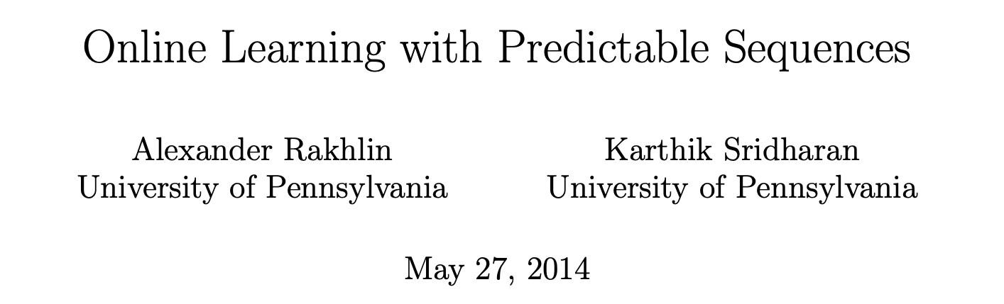
3. Found a relevant article on regret bounds for "predictable sequences".
Maybe I can borrow some ideas ?
- At round t,
- Learner picks an action \( f_t \in \mathcal{F} \),
- Nature reveals \( x_t \in \mathcal{X} \),
- learner suffers loss \( \langle f_t, x_t \rangle \). - Goal : Minimize regret against the best fixed action in hindsight:
\( \mathrm{Reg}_T = \sum_{t=1}^T \langle f_t, x_t \rangle - \inf_{f \in \mathcal{F}} \sum_{t=1}^T \langle f, x_t \rangle \)
Online Learning with Predictable Sequences
Online Linear Optimization Setting
Mirror Descent, FTRL etc. guarantee \( \mathrm{Reg}_T = O(\sqrt{T}) \) regardless of the sequence.
Tight for adversarial sequences but pessimistic when the sequence has structure
Online Learning with Predictable Sequences
Assume that the sequence is benign: well described by a predictable process
\[ M_t(x_1, \ldots, x_{t-1}) \]such that
\[ x_t = M_t + \delta_t \] where \( M_t \) is a fixed guess and \( \delta_t \) is small noise.
The learner uses \( M_t \) as an internal hint to compute a better action at each round.
Examples:
1. \( M_t = x_{t-1} \) (path-length),
2. \( M_t = \frac{1}{t-1}\sum_{s<t} x_s \) (empirical mean), or any auto-regressive model.
3. \( M_t = \frac{1}{t-1}\sum_{s<t} \alpha_s x_s \), where \(\sum_{s}\alpha_s = 1\). "fading memory statistics"
Can we incorporate prior information on the evolution of sequence into regret analysis?
Online Learning with Predictable Sequences
"Optimistic Mirror Descent" algorithm incorporates \( M_{t+1} \) into the update as if it were the true next move:
The main regret bound (Lemma 2) is:
\[ \mathrm{Reg}_T \leq \frac{(\text{Diam}(\mathcal{F}))^2}{\eta} + \frac{\eta}{2} \sum_{t=1}^T \|x_t - M_t\|_*^2 \quad \xrightarrow{\text{optimize } \eta} \quad \mathrm{Reg}_T \leq c\,\sqrt{\sum_{t=1}^T \|x_t - M_t\|_*^2} \]
- If \( x_t = M_t \) exactly, regret is zero. For low-variance i.i.d. data with noise \( \sigma \), regret becomes \( O(\sigma\sqrt{T}) \), vanishing as \( \sigma \to 0 \).
- Crucially, the bound degrades gracefully: if \( M_t \) predicts poorly, \( \sum_t \|x_t - M_t\|^2 \leq 4T \), recovering \( O(\sqrt{T}) \) up to a constant factor.
Pretend that \(M_{t+1}\) is the correct generator for \(x_{t+1}\)
Authors also discuss "learning" \(M_t \in \mathcal{M}\), but that incurs a log-cost in the regret bound \( \log |\mathcal{M}| \)
1. Sent slides on Learned DA
2. Readings on cutting edge methods in Video-SR.
3.
March 5
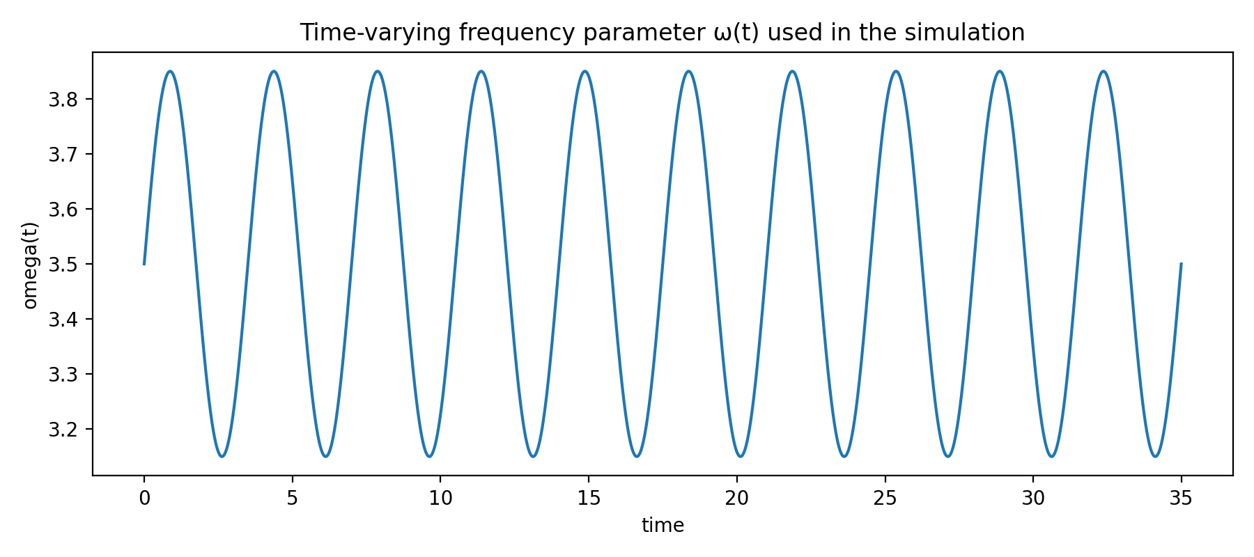
\(α = 0.95,\; β = 0.7,\; λ = 0.6,\; ω(0) = 3.5,\; ρ =0.25, ε = 0.1\)
Langford dynamical system
Varying \(\omega\)
sinusoidally
Langford dynamical system
Still working on theory
Each observation has imperfect information on the phase because of noise.
Tracking phase through history via a filtering algorithm can help, but windowing throws away information
Langford dynamical system
Tracking amplitude and phase enables form full history can be better
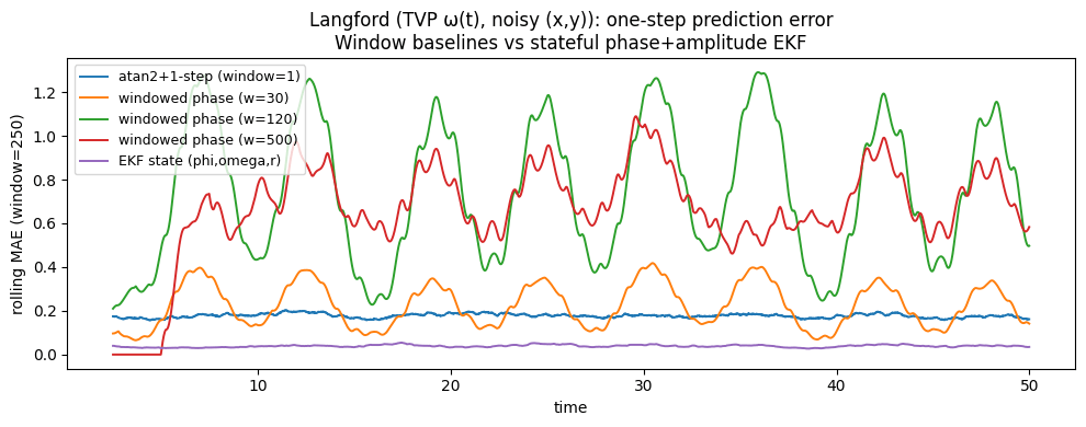
Window algorithm : estimate phase, amplitude from window (length \(w\))
EKF : track phase, amplitude as "states" and predict \(y_{t+1}\)
12/18
Title Text
- Bullet One
- Bullet Two
12/5/25
Diffusion-based DA with dynamical guidance
Given \( \{x_t^{ref}, y_t\}_{t=1}^T\), learn:
-
A forward model F that captures the dynamics of state evolution.
-
An analysis model G that assimilates the forecasted state and the new observation to produce an updated estimate (the analysis state). Formally, a conditional denoising diffusion model.
generated distribution with conditioning
Diffusion-based DA with dynamical guidance
At inference time, given \(x_0\) and \( \{y_1, y_2, \ldots \} \)
- Generate \(x_1^A \sim G(x_0, y_1)\)
- Forecast \( x_2^F = F(x_1^A) \)
- Analyze \( x_2^A \sim G(x_2^F, y_2) \)
Experiment with different diffusion models and different ground truth dynamics
Diffusion-based DA with dynamical guidance
Supervised learning objective
Generative model explicitly incorporates dynamics through conditioning on forecast state.
prediction from reference
Diffusion-based DA with dynamical guidance
I propose that we enforce more regularity during training
analysis for time t from \(x_t^{F,ref}\)
Enforce additional forward constraints
Implicitly asks F, G to be aligned
Diffusion-based DA with dynamical guidance
Regularity for analysis model
Backward alignment.
Conditioned on \(y_t\) if the predicted state resembles state at next time step, then generative model should still sample near \(x_t^{ref}\)
Diffusion-based DA with dynamical guidance
Learning objectives
Learn forward from data
Learn to analyze from data
forward and analysis should align
Analysis should be
backwards compatible
Diffusion-based DA with dynamical guidance
These constraints can be approximately specified for the denoiser network.
12/4/25
I proposed an algorithm where forward dynamics and analysis step are jointly learned from (state,observation) trajectories.
Two main questions from last meeting:
-
Why not particle filters?
A vague answer : particle filters might not scale well
a. weight degeneracy in high dimensions.
b. high accuracy might need a large number of particles
-
How does the proposal relate to other approaches?
A vague answer : Accounting for dynamics by jointly learning should be better for assimilation.
Many recent articles propose to replace the entire DA frameworks with generative models (mostly diffusion)
Rozet and Louppe 2023; Chung et al. 2023; Manshausen et al. 2024; Pathak et al. 2024; Qu et al. 2024; Li et al. 2025)
Readings on improving the analysis step in DA
-
A diffusion model is learned to denoise noisy states while conditioned on the observation.
- Often training data = state and observations pairs.
1. sometimes a full trajectory
2. sometimes proxy of states based on different physical models
3. sometimes based on the output of a different DA method.
- During assimilation, given an observation \(y\), we can recover the state by sampling from \(p(x|y)\) using reverse-diffusion SDE
-
Different diffusion-based DA systems learn different Bayesian posterior distributions. Hodyss et. al, 2025 claim that diffusion models that account for forward dynamics are better based on simplified experimental settings (linear, Gaussian)
Diffusion models for DA
1. Climatology-trained diffusion DA
- Training data = long historical trajectories \(\{x_t, y_t\}\). Roughly equivalent to samples from a steady-state joint distribution called the climatological prior : \( p_{\text{clim}}(x)\).
- Diffusion model samples from \( p(x_t \mid y_t) \propto {\color{blue} p_{\text{clim}}(x_t)}\, p(y_t \mid x_t).\)
2. Cycle-trained diffusion DA
- Retrain the diffusion model in each DA cycle with a new generated dataset.
- Start with multiple trajectories, propagate to desired time step. Train diffusion model for the specific time step
- Diffusion model samples from \(p(x_t \mid y_t) \propto {\color{blue} p(x_t \mid y_{1:t-1})} \, p(y_t \mid x_t).\)
-
Cycle-trained diffusion makes little sense to me given the need to retrain. Hodyss et. al. 2025 claim this cumbersome procedure is better
3. Hybrid diffusion DA
- Forward propagation either using a physical model, NN, or a diff DA method.
- Training data uses forecast states \(x_t^{f} \sim p_{\text{model}}(x_t \mid x_{t-1})\) paired with observations. The diffusion model samples from \(p(x_t \mid y_t) \propto {\color{blue} p_{\text{model}}(x_t \mid y_{1:t-1})}\, p(y_t \mid x_t).\)
A rough taxonomoy of diffusion-based DA
Method : Represent the filtering density \(p(x_t|y_t)\) via a score-based diffusion model instead of a finite particle set.
-
Each DA step: propagate previous states through the known dynamics, retrain the score network on these samples to approximate the prior filtering density \(p(x_t|y_1, \ldots, y_{t-1})\) .
-
Update the score function analytically from prior filtering density to posterior filtering density
-
Sampling: draw arbitrarily many samples from the filtering density with the reverse-time diffusion using the learned score.
Key : Dynamics are not learned. Score function is continuously updated and retrained through DA.
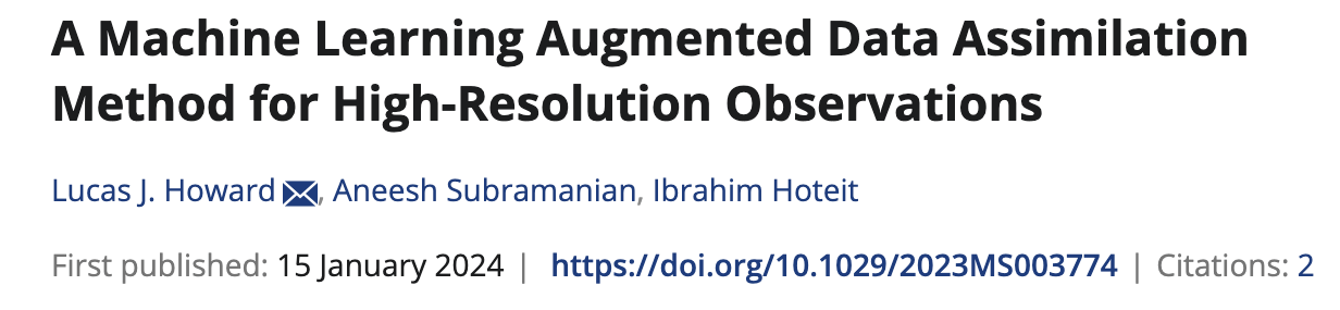
A score-based filter for nonlinear data assimilation
Journal of Computational Physics, Oct 2024
-
Training data: State–observation trajectories \(\{x_k, y_k\}_{k=1}^K\)
-
Learning Task: A conditional diffusion model of the smoothing posterior \(p(x_{1:K} | y_{1:K})\) p(x1:K∣y1:K)p(x_{1:K} \mid y_{1:K}).
-
Contribution: Non-linear observation operators are handled by doing DA for the pair of augmented state \(z=(x,y)\) and observations \(y\).
State-Observation Augmented Diffusion (SOAD) model for nonlinear assimilation with unknown dynamics
Journal of Computational Physics , Oct 2025
11/20/25
Updates
- Reading more literature on analysis operators. Aiming to have a share-able document on Monday, Dec 1.
Both articles learn analysis operator in somewhat similar manner
- Applying to more TT' jobs now
- Assembling my application materials
- Still polishing my research statement
11/13/25
Dynamical system
state evolution
observations
1. When \(\epsilon_t, \eta_t\) is Gaussian (and independent of state iterates), Kalman filter is optimal.
2. Analysis filter in KF is linear in the predicted state \(u_t^f\) and observation \(y_t\)
Goal : improve analysis step
Suppose we have a batch of paired state, observations
$$(u_t^{ref}, y_t)$$
where \(u_t^{ref}\) is the reference state at time t, for eg,
1. accurate but computationally intensive high-fidelity numerical solvers,
2. high-quality reanalysis products (e.g., ERA5 for global atmospheric circulation),
A proposal
- Learn a forward model \(F_{\theta}\) for state dynamics:
- Learn an analysis step in two sub-parts.
2.1 A course deterministic operator \(T_{\psi}\) such that:
2.2 A fine-grained probabilistic analysis operator \(p_{\phi}\) that learns the residual
Prediction step
Analysis step 1
Analysis step 2
deterministic, coarse
probabilistic, finer
where, \(r_t \sim p_{\phi}(y_t, \tilde{u}_t)\)