Introduction to
Bayesian Optimization
Roberto Calandra
Facebook AI Research
CS188 - UC Berkeley - 10 April 2020
Goals of the Lecture
- Being familiar with the relevant Bayesian optimization (BO) notation
- Know how BO works
- Understand strengths and limitations of BO
- Being aware of several real-world applications which use BO
- (Understand at the high-level how Gaussian processes work)
- (Recognize the similarities to the MDP formulation and RL)
- (Familiarize with the basic formulation of multi-objective optimization)
Black-box Optimization
Optimized parameters
Objective function
Parameters to optimize
A Taxonomy of Objective Functions
Single minimum
(e.g., convex functions)
Multiple minimum
(a.k.a., global optimization)
First-order
(we can measure gradients)
Zero-order
(no gradients available)
Noise-less
(repeating the evaluation yield the same result)
Stochastic
(repeating the evaluation yield different results)
Nice and easy to solve
(e.g., with gradient descent)
Cheap Evaluation
(virtually infinite number of evaluations allowed)
Difficult to optimize!
Expensive Evaluation
(limited to tens or hundreds of evaluations)
Examples of Expensive Optimization
Oil drilling
Design and manufacturing
Drug design
Robotics
Hyperparameters optimization


Hyperparameters Optimization
- Machine learning models are growing more and more complex
- Modern deep learning models have dozens of hyperparameters that need to be tuned (e.g., learning rates, number of layers, batch size...)
- To achieve state-of-the-art results, finding good hyperparameters is crucial
- However, even for experts finding good hyperparameters can be difficult and time consuming
- How can we automatically optimize them?
Vibrant community dedicated to automated machine learning (AutoML)
Traditional Optimization Approaches
- Manual tuning (requires expert knowledge)
- Grid Search (does not scale to large parameter spaces)
- Random Search (better than grid search, but still too many evaluations)
- Gradient descent (only feasible for first-order functions)
- Evolutionary strategies (requires thousands of evaluations)
- ...
With dozens of parameters, complex correlations, and expensive evaluations
these methods become impractical
Intuition Behind Bayesian Optimization
- Many optimizers capture only local information about the objective function
- Can we instead use all information (i.e., the evaluations) collected so far to make a more informed decision, hence improving data-efficiency?
- How to do this in practice?
e.g.,
We can create a surrogate model
Gradient descent
Bayesian Optimization
- Learn response surface
- Based on the response surface, select next parameters to evaluate
- Evaluate
on the objective function - Repeat until stop criteria


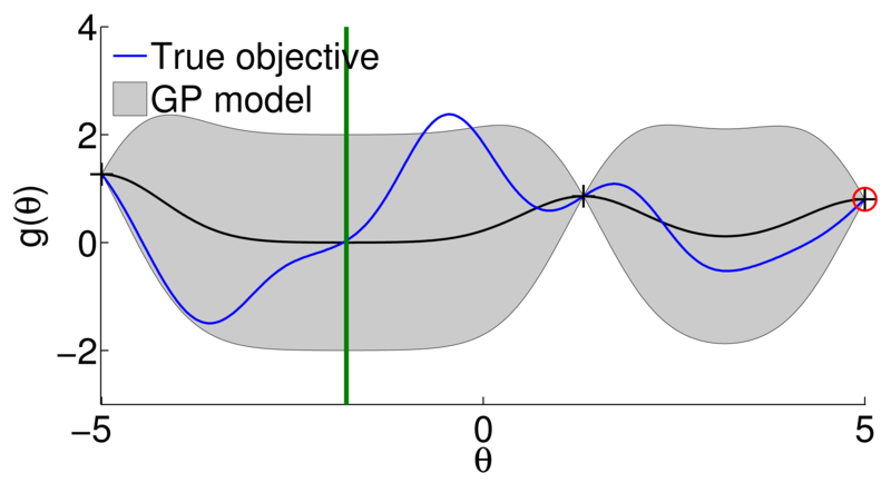


[credit: Marc Deisenroth]


Questions ?
Brief History of BO & Related Fields
- Independently "re-invented" over and over throughout the last 50 years in different communities.
- [Krige 1951] Widely adopted in geostatistics under the name of "Kriging"
- [Kiefer 1959] as optimum experimental designs
- [Kushner 1964]
- [Mockus 1978]
- [Jones 1998 ] as Efficient Global Optimization (EGO)
- BO can be considered a continuous version of the "multi-armed bandit" problem
- BO can also be considered a policy search algorithm
(family of reinforcement learning algorithms) - Main difference with reinforcement learning is that BO formulation does not have a state that changes over time
Response Surface
Large variety of models used throughout the literature:
- Polynomial functions
- Random forests
- Bayesian neural networks
- Gaussian processes
- ...
By far the most commonly used (currently)
Surrogate model (a.k.a. response surface) need to accurately approximate (and generalize) the underlying function based on the available data
Gaussian Processes
Additional reading:
Rasmussen, C. E. & Williams, C. K. I.
Gaussian Processes for Machine Learning
The MIT Press, 2006
- Distribution over functions
- Probabilistic Model
Mean of a GP = Kernel ridge regression
- The posterior predictive distribution for an arbitrary input is computed as:
- Flexible Bayesian regression method
Intuition of Gaussian Processes


Covariance Functions and GP Training
Square exponential
parameters of the GP
(often referred to as hyperparameters)
Multiple ways to optimize the hyperparameters
- MAP estimate (by optimizing marginal likelihood)
- Numerical integration (proper Bayesian way, but often more complicated)
Additional reading:
Rasmussen, C. E. & Williams, C. K. I.
Gaussian Processes for Machine Learning
The MIT Press, 2006
Why Gaussian Processes?
Pro:
- Mathematically well-understood
- Calibrated uncertainties
- Possibility of specifying priors (e.g., of the underlying function)
- Easy to enforce Lipschitzian smoothness (by choosing appropriate kernel)
- Good modeling capabilities in low-data regime
Cons:
- Difficult to scale to high-dimensional input space
- Computationally expensive
- Quality of the model dependent from use of appropriate kernel
Acquisition Function
- How do we select the next parameters to evaluate?
- Intuition: A good acquisition function need to strike a smart balance between exploration and exploitation
-
Many acquisition functions in the literature:
- Probability of improvement
- Expected improvement
- Upper confidence bound
- Entropy search
- Predictive entropy search
- ...
Optimizing the Acquisition Function
- Optimizing the acquisition function is by itself a challenging optimization problem.
- However:
- No longer stochastic
- No longer zero-order
(We can usually compute gradients and Hessian of the acquisition function) - Not expensive to compute
(Although potentially computationally intensive)
- Often global optimization methods are used (e.g., CMA-ES or DIRECT) followed by a first-order optimizer (e.g., gradient descent)
Recap

Questions ?
Extensions of Standard BO
Numberless extensions in the literature:
- Constrained optimization (linear and non-linear constraints)
- Multi-task optimization (we can exploit the statistical correlation to previously optimized tasks)
- Robust optimization
- Safe optimization
- Batch optimization (several parameters are evaluated at once)
- Contextual optimization (more about this soon)
- Multi-objective optimization (more about this soon)
- Grey-box optimization
- ...
Contextual Bayesian Optimization
Optimized parameters
Objective function
Parameters to optimize
Context
Contextual Bayesian Optimization
- Very common case
- Striking similarities with RL -- context is akin to the state in an MDP
- Minimal changes to the basic BO algorithm:
- Response surface is now
- The optimization of the acquisition function becomes constrained
Multi-objective Bayesian Optimization
- Most engineering problems are truly multi-objective

Pareto Front
- Not all objective functions can be optimized at once
- Solving this optimization means finding the
Multi-objective Bayesian Optimization
- Multi-objective BO aims at finding the Pareto Front in a data-efficient manner
- Common way to solve is to scalarize the multiple objectives into a single one
[Knowles, J. ParEGO: A hybrid algorithm with on-line landscape approximation for expensive multiobjective optimization problems IEEE Transactions on Evolutionary Computation, 2006, 10, 50-66]
- For example, by using a Tchebycheff scalarization
Questions ?
Learning to Walk using BO


Bio-inspired Bipedal Robot "Fox":
- Quasi-passive dynamic walker
- 4 Degrees of freedom
- Springs in legs
- Walking in circle
- Finite-state-machine controller (from biomechanics)
- 8 parameters
- (Motors life ~200 trials)
[Calandra, R.; Seyfarth, A.; Peters, J. & Deisenroth, M. P. Bayesian Optimization for Learning Gaits under Uncertainty Annals of Mathematics and Artificial Intelligence (AMAI), 2015, 76, 5-23]
Learning to Walk in 80 Trials
[Calandra, R.; Seyfarth, A.; Peters, J. & Deisenroth, M. P. Bayesian Optimization for Learning Gaits under Uncertainty Annals of Mathematics and Artificial Intelligence (AMAI), 2015, 76, 5-23]
Learning Curve - Fox

[Calandra, R.; Seyfarth, A.; Peters, J. & Deisenroth, M. P. Bayesian Optimization for Learning Gaits under Uncertainty Annals of Mathematics and Artificial Intelligence (AMAI), 2015, 76, 5-23]
Learned model


Not Symmetrical (about 5° difference). Why?
Because it is walking in a circle!
[Calandra, R.; Seyfarth, A.; Peters, J. & Deisenroth, M. P. Bayesian Optimization for Learning Gaits under Uncertainty Annals of Mathematics and Artificial Intelligence (AMAI), 2015, 76, 5-23]
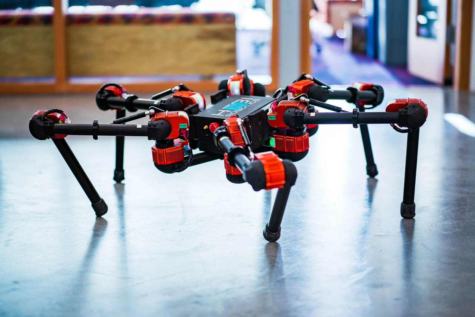
Example of Multi-objective BO


Simulated hexapod:
- 12 Degrees of Freedom (2 per legs)
- No good physics models at that scale
- we use Central Pattern Generators (CPG) as controllers
[Yang, B.; Wang, G.; Calandra, R.; Contreras, D.; Levine, S. & Pister, K. Learning Flexible and Reusable Locomotion Primitives for a Microrobot IEEE Robotics and Automation Letters (RA-L), 2018, 3, 1904-1911]
Hard-coded CPG Gaits

[Yang, B.; Wang, G.; Calandra, R.; Contreras, D.; Levine, S. & Pister, K. Learning Flexible and Reusable Locomotion Primitives for a Microrobot IEEE Robotics and Automation Letters (RA-L), 2018, 3, 1904-1911]
Single-objective


[Yang, B.; Wang, G.; Calandra, R.; Contreras, D.; Levine, S. & Pister, K. Learning Flexible and Reusable Locomotion Primitives for a Microrobot IEEE Robotics and Automation Letters (RA-L), 2018, 3, 1904-1911]
Dual Tripod Gait
[Yang, B.; Wang, G.; Calandra, R.; Contreras, D.; Levine, S. & Pister, K. Learning Flexible and Reusable Locomotion Primitives for a Microrobot IEEE Robotics and Automation Letters (RA-L), 2018, 3, 1904-1911]
Multi-objective


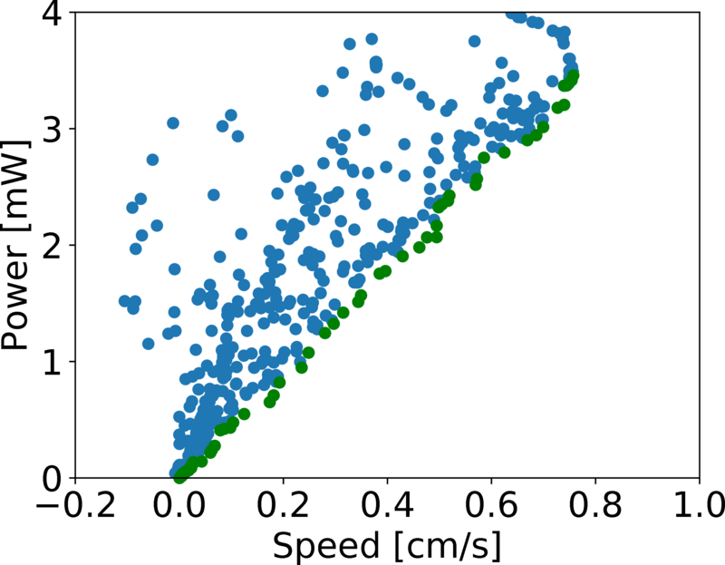

[Yang, B.; Wang, G.; Calandra, R.; Contreras, D.; Levine, S. & Pister, K. Learning Flexible and Reusable Locomotion Primitives for a Microrobot IEEE Robotics and Automation Letters (RA-L), 2018, 3, 1904-1911]
Comparison Gaits

[Yang, B.; Wang, G.; Calandra, R.; Contreras, D.; Levine, S. & Pister, K. Learning Flexible and Reusable Locomotion Primitives for a Microrobot IEEE Robotics and Automation Letters (RA-L), 2018, 3, 1904-1911]
Discovering New Gaits

[Yang, B.; Wang, G.; Calandra, R.; Contreras, D.; Levine, S. & Pister, K. Learning Flexible and Reusable Locomotion Primitives for a Microrobot IEEE Robotics and Automation Letters (RA-L), 2018, 3, 1904-1911]
Example of Contextual BO

[Yang, B.; Wang, G.; Calandra, R.; Contreras, D.; Levine, S. & Pister, K. Learning Flexible and Reusable Locomotion Primitives for a Microrobot IEEE Robotics and Automation Letters (RA-L), 2018, 3, 1904-1911]
Limitations of Bayesian Optimization
- Surprisingly efficient in many applications
- Easy to include more structure/priors/past evaluations for a given problem
- Interpretable models can provide insight
- It works in the real-world !
- Does not scale to high-dimensional parameter space
(~30-D for Gaussian processes, and a few hundred with more structured models) - No guarantees of convergence
- If the underlying function is difficult to model, it often results in poor performance
(e.g., discontinuous functions, or with a lot of local minima)
Summary
- Bayesian optimization is a popular tool for global optimization of expensive black-box functions
(Many engineering problems can be reliably solved by BO) - Introduced standard BO notation
- Presented BO algorithms and its components
- Briefly discussed special instances of BO (contextual and multi-objective)
- Described strengths and limitations of BO
- Examples from real-world applications of BO
- BO is a very active field of research
Please give Feedback at: https://tinyurl.com/cs188introbo

References
- Brochu, E.; Cora, V. M. & De Freitas, N.
A tutorial on Bayesian optimization of expensive cost functions, with application to active user modeling and hierarchical reinforcement learning
arXiv preprint arXiv:1012.2599, 2010 -
Shahriari, B.; Swersky, K.; Wang, Z.; Adams, R. P. & de Freitas, N.
Taking the human out of the loop: A review of Bayesian optimization
Proceedings of the IEEE, IEEE, 2016, 104, 148-175 -
Rasmussen, C. E. & Williams, C. K. I.
Gaussian Processes for Machine Learning
The MIT Press, 2006 - Calandra, R.; Seyfarth, A.; Peters, J. & Deisenroth, M. P.
Bayesian Optimization for Learning Gaits under Uncertainty
Annals of Mathematics and Artificial Intelligence (AMAI), 2015, 76, 5-23 - Yang, B.; Wang, G.; Calandra, R.; Contreras, D.; Levine, S. & Pister, K.
Learning Flexible and Reusable Locomotion Primitives for a Microrobot
IEEE Robotics and Automation Letters (RA-L), 2018, 3, 1904-1911 - Kushner, H. J.
A new method of locating the maximum point of an arbitrary multipeak curve in the presence of noise
Journal of Basic Engineering, 1964, 86, 97-106 - Mockus, J.; Tiesis, V. & Zilinskas, A.
The application of Bayesian methods for seeking the extremum
Towards Global Optimization, Amsterdam: Elsevier, 1978, 2, 117-129 - Jones, D. R.; Schonlau, M. & Welch, W. J.
Efficient global optimization of expensive black-box functions
Journal of Global Optimization, Springer, 1998, 13, 455-492 -
Knowles, J.
ParEGO: A hybrid algorithm with on-line landscape approximation for expensive multiobjective optimization problems
IEEE Transactions on Evolutionary Computation, 2006, 10, 50-66 -
Hutter, F.; Hoos, H. H. & Leyton-Brown, K.
Sequential model-based optimization for general algorithm configuration
Learning and Intelligent Optimization (LION), Springer, 2011, 507-523 -
Snoek, J.; Larochelle, H. & Adams, R. P.
Practical Bayesian Optimization of Machine Learning Algorithms
arXiv preprint arXiv:1206.2944, 2012
Credits
- Page 5: image oil drill - CGP Grey (https://flic.kr/p/8s4LXw) - CC BY 2.0
- Page 5: image drug design - Jamie (https://flic.kr/p/9KVkMX) - CC BY 2.0
- Page 5: image Design and manufacturing - Michele Mischitelli (https://flic.kr/p/2hv3RWE) - CC BY-ND 2.0
- Page 5: image hyperparameters optimization - Samuel Humeau, Kurt Shuster, Marie-Anne Lachaux, Jason Weston - Poly-encoders: Transformer Architectures and Pre-training Strategies for Fast and Accurate Multi-sentence Scoring
- Page 5: image robot - Facebook
- Page 8: images BO - Marc Deisenroth