Hydrogen transport in tokamaks
Estimation of the ITER divertor tritium inventory and influence of helium exposure
Rémi Delaporte-Mathurin
17-10-2022



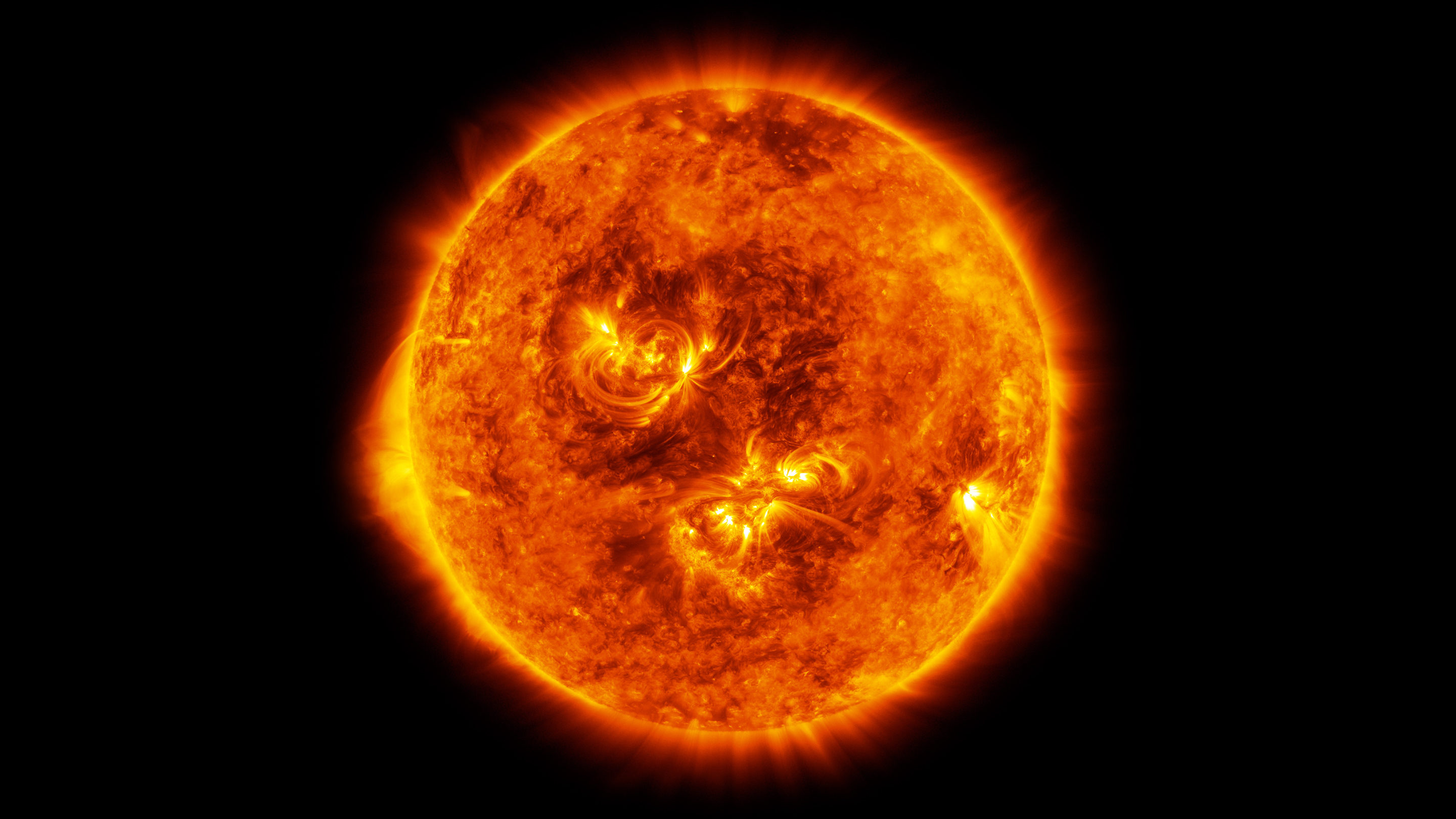
“I’d put my money on the Sun. What a source of power!”
Thomas Edison, 1931
Every second:
→ Fuses 500 Mt of hydrogen
→ Produces a million times the world’s energy consumption
On Earth
Deuterium
Tritium
Neutron
Helium
✔️No CO2 emission
✔️No long lived radioactive waste
✔️Inherently safe
✔️Abundant fuel

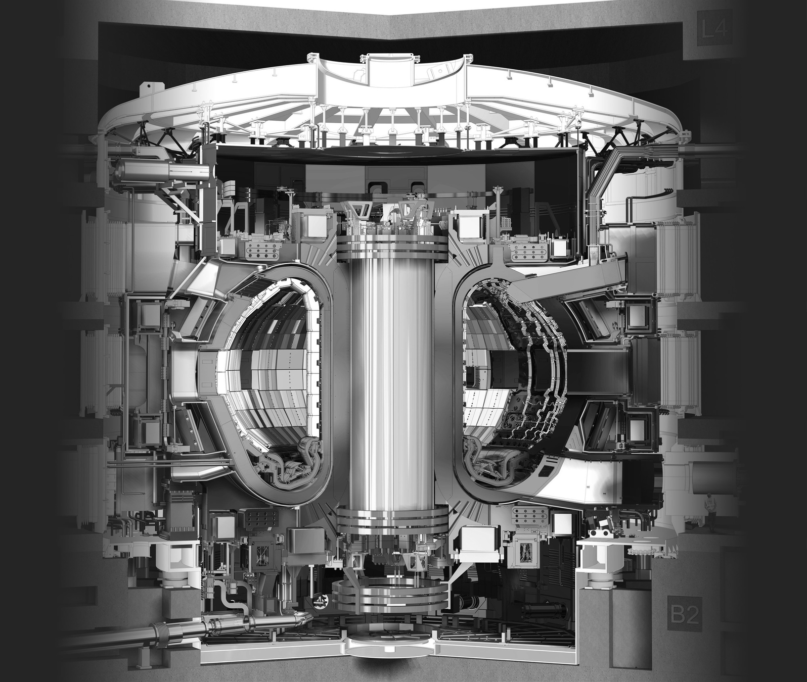
ITER



Plasma: mixture of Hydrogen (D-T) and Helium
Particle bombardment
Divertor


Why should we care?
T is rare
T is expensive
€£$
Material embrittlement
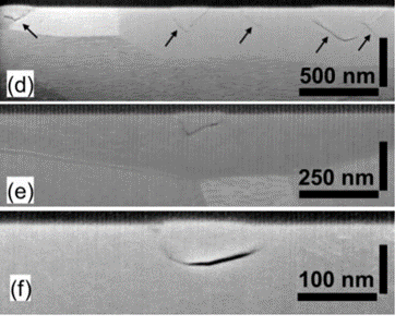
Gao et al, Nucl Fusion (2019)
What's the T inventory in the ITER divertor?
Does it remain within safety limits?
What's the influence of Helium?
T is radioactive
☢


Why should we care?
T is rare
T is expensive
£
Material embrittlement

T is radioactive

Gao et al, Nucl Fusion (2019)
What's the T inventory in the ITER divertor?
Does it remain within safety limits?
What's the influence of Helium?
Material embrittlement

Gao et al, Nucl Fusion (2019)
Fuel recycling

£
☢

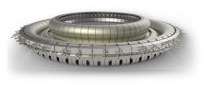
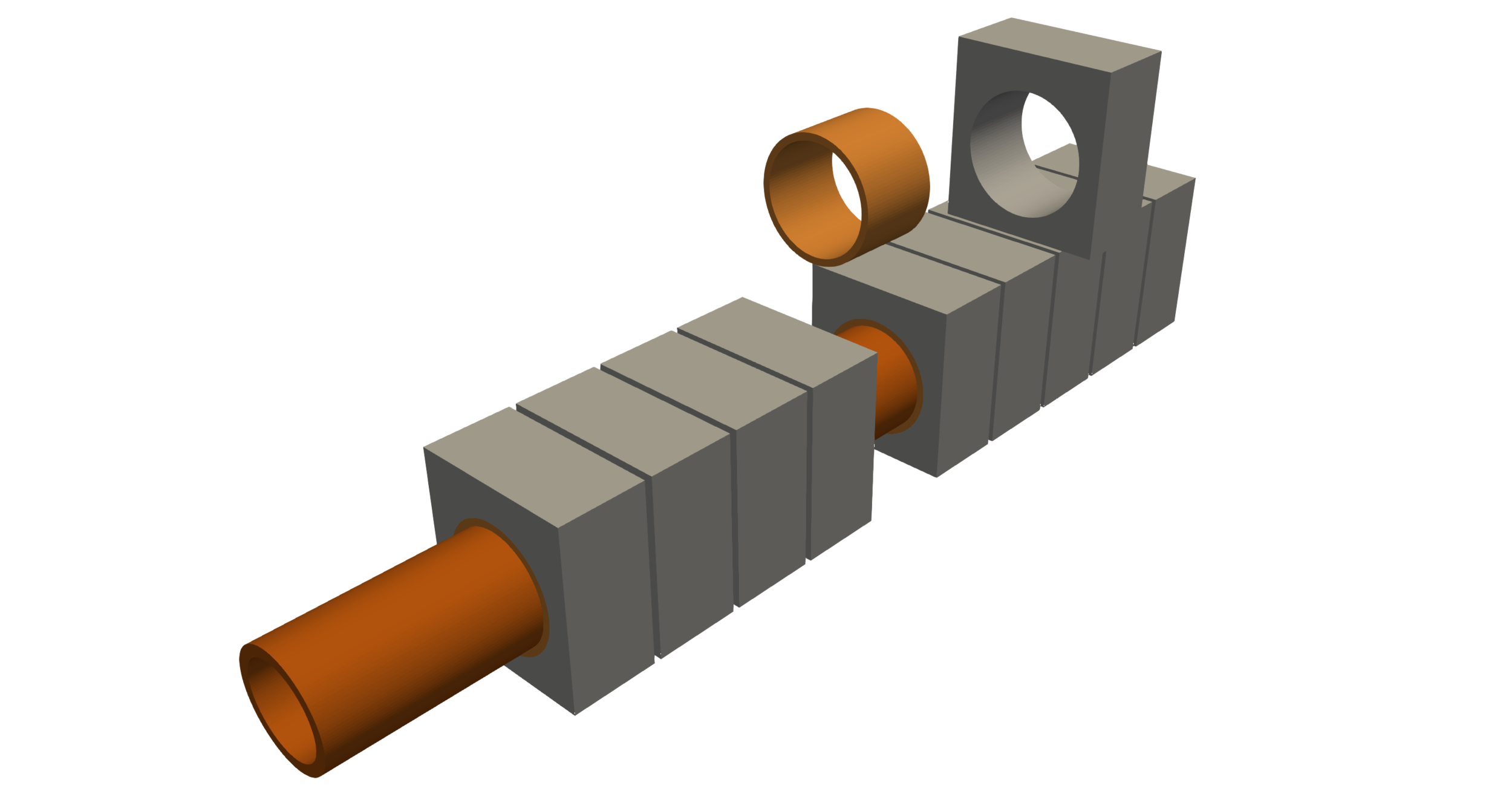
W
Cu
CuCrZr
Monoblocks

W
Cu
CuCrZr
Monoblock
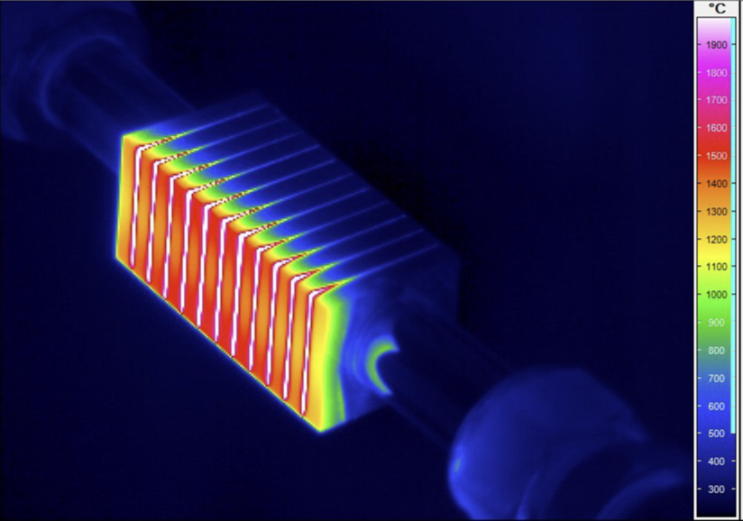
Top surface exposed to extreme fluxes (particle, heat)


Pressurised water convection
14 mm
Outline
- Assessment of the tritium inventory in the ITER divertor
- Models & tools
- Monoblocks
- Divertor
- Influence of helium impurities
- Helium bubble model
- Interactions with hydrogen transport


Models and tools
Hydrogen transport in metals

H transport equations

Fick's law
H transport equations

concentration of mobile hydrogen
Fick's law
H transport equations

concentration of mobile hydrogen
diffusion coefficient
Fick's law
H transport equations

McNabb & Foster
H transport equations

concentration of trapped hydrogen
McNabb & Foster
H transport equations

trap concentration
concentration of trapped hydrogen
McNabb & Foster
H transport equations

trap concentration
concentration of trapped hydrogen
McNabb & Foster
trapping rate
detrapping rate
H transport equations
Conservation of chemical potential at interfaces
Material 1
Material 2
\( c_\mathrm{m} \)
\( S\): solubility of H in the material
H transport equations
\( \textcolor{red}{T} \) : Temperature (K)
Thermally activated coefficients
\( D = D_0 \exp(-E_D / k_B \textcolor{red}{T}) \)
\( k_i = k_0 \exp(-E_k / k_B \textcolor{red}{T}) \)
\( p_i = p_0 \exp(-E_p / k_B \textcolor{red}{T}) \)
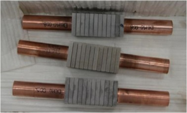
1800 °C
300 °C
20 MW/m2
\(k_B \): Boltzmann constant
We also need the heat equation
thermal conductivity
heat capacity
density

Wishlist
- Multi-materials
- Multi-dimensional
- Hydrogen transport
- Heat transfer
| 1D H transport | 2D/3D | Multi-material | Heat transfer | |
|---|---|---|---|---|
| TMAP7 | ✓ | ✓ | ||
| HIIPC | ✓ | ✓ | ||
| CRDS | ✓ | |||
| MHIMS | ✓ | |||
| TESSIM | ✓ | ✓ | ||

Wishlist
- Multi-materials
- Multi-dimensional
- Hydrogen transport
- Heat transfer
| 1D H transport | 2D/3D | Multi-material | Heat transfer | |
|---|---|---|---|---|
| TMAP7 | ✓ | ✓ | ||
| HIIPC | ✓ | ✓ | ||
| CRDS | ✓ | |||
| MHIMS | ✓ | |||
| TESSIM | ✓ | ✓ | ||
| FESTIM | ✓ | ✓ | ✓ | ✓ |
FESTIM implements these models
FESTIM
Finite element
H transport
Heat transfer
Complex geometries

The finite element method
Steady state weak formulation:
Transient weak formulation:
In FESTIM
Type of finite elements:
- P1 (CG1) for \( c_\mathrm{m} \)
- P1 or DG1 for \( c_\mathrm{t, i} \)
FESTIM: a code verified & validated
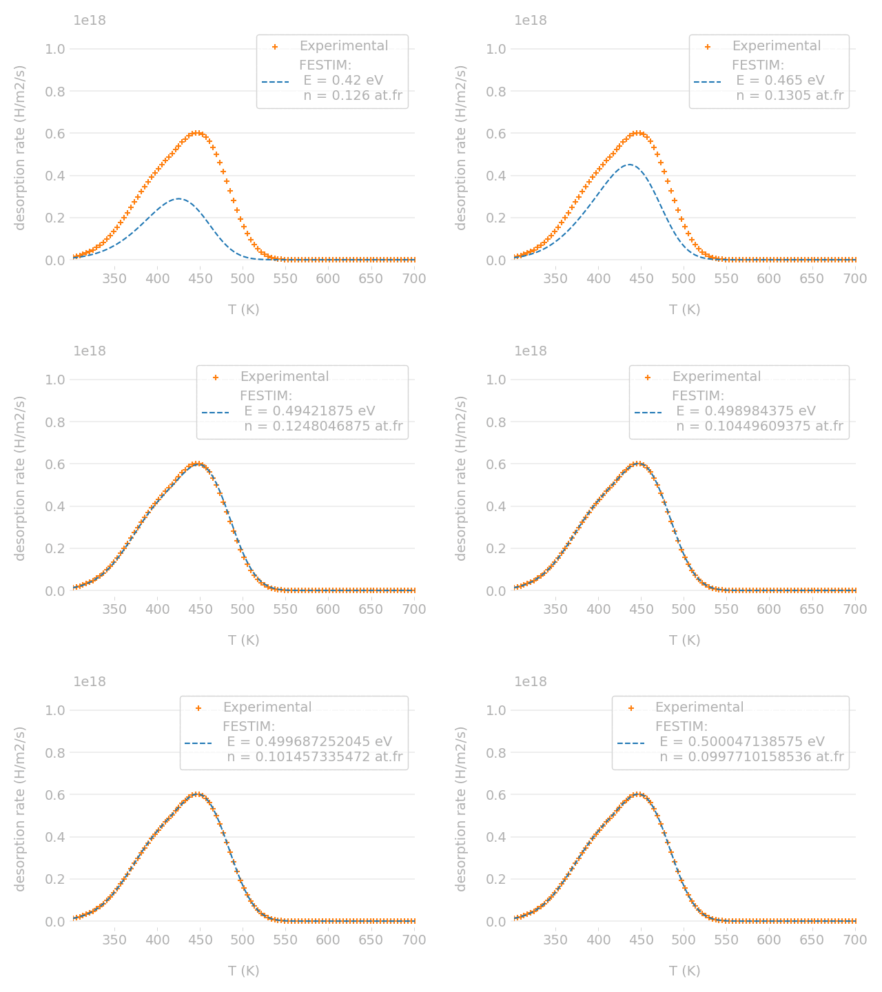
Experimental validation
Analytical verification
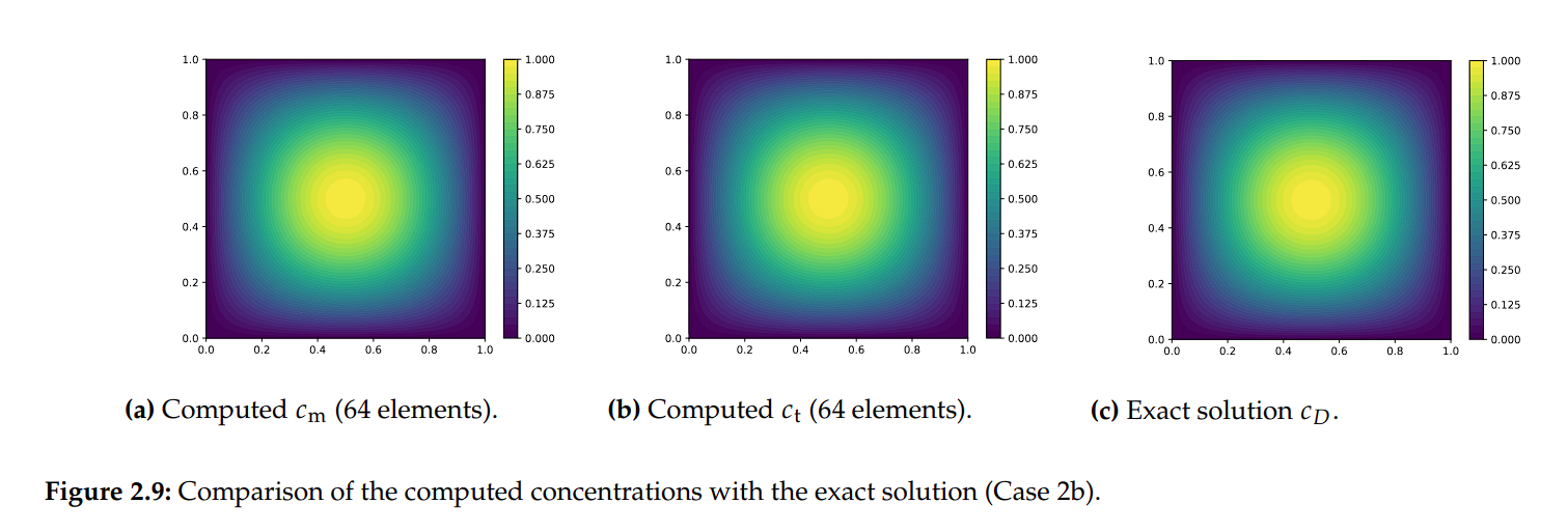
Exact
Computed concentration
Parametric optimisation technique

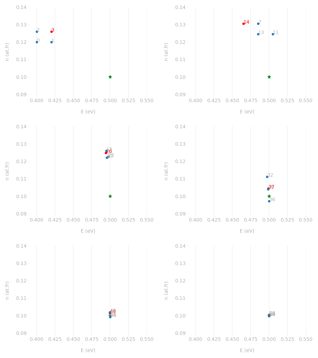
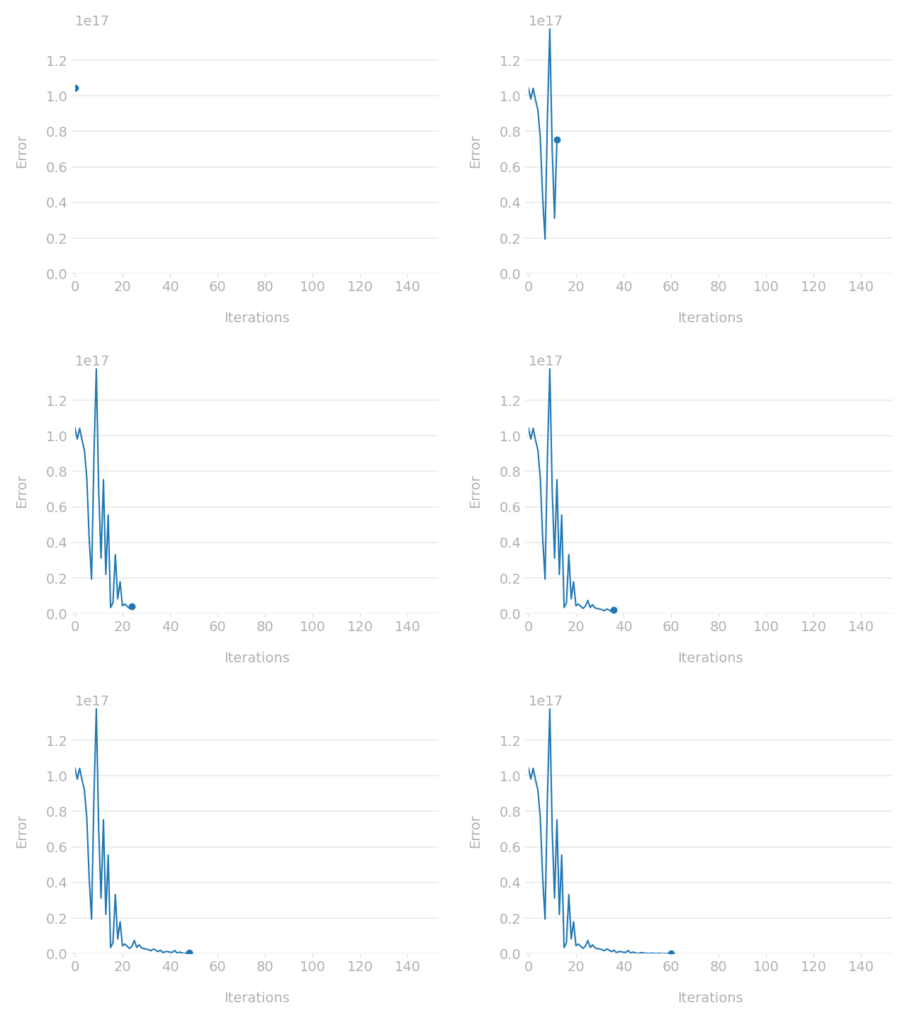
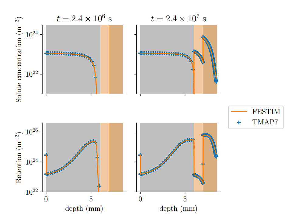
Cross-check with TMAP7
FESTIM main features
Physics
- Hydrogen diffusion
- Trapping (McNabb & Foster)
- Heat transfer
- Conservation of chemical potential
- Soret effect
Dimension
✅ 1D
✅ 2D
✅ 3D
Boundary conditions
- Imposed concentration/temperature
- Hydrogen/heat flux
- Recombination flux
- Dissociation flux
- Convective heat flux
- Sievert's law
- Plasma implantation approx.
- ...
Traps
- Time/space dependent densities
- Extrinsic traps
FESTIM: an open-source code
✅ More transparency
✅ More collaborations
✅ More flexibility
Automated documentation
FESTIM workshop
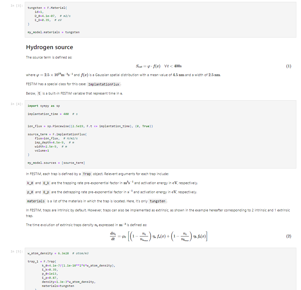
A FESTIM course to learn how to run H transport simulations
Monoblock simulations
FESTIM model
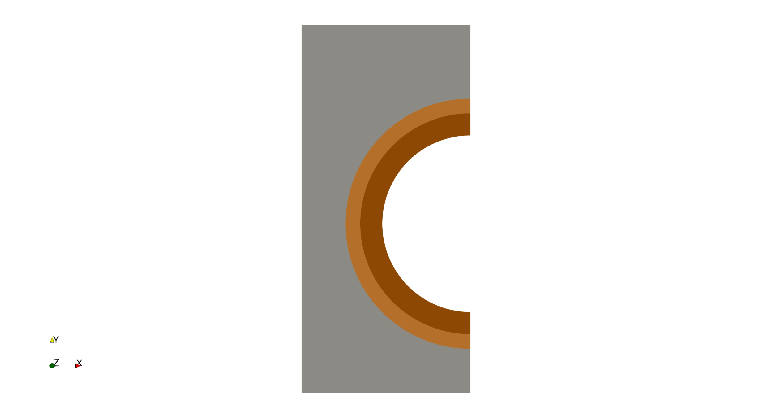
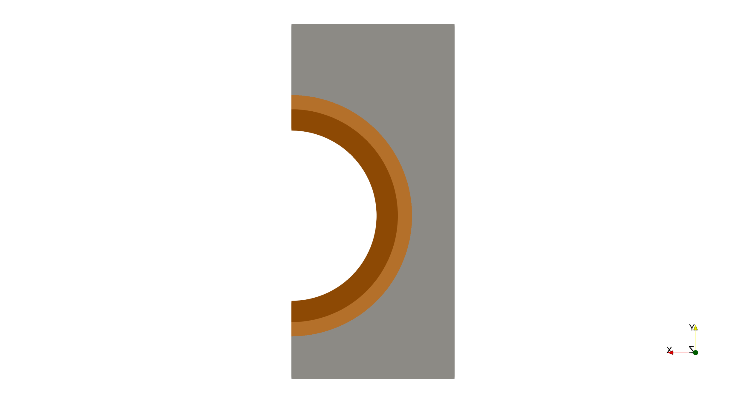
Heat flux \( \varphi_\mathrm{heat} \)
Imposed concentration
Convection
H recombination
Conservative assumptions:
- 2D
- Continuous exposure
- No desorption on gaps
Influence of mechanical fields neglected

Boundary conditions
Convective flux: \( -\lambda \nabla T \cdot n = h \ (T-T_\mathrm{coolant}) \)
Recombination flux: \( -D \nabla c_\mathrm{m} \cdot n = K_r \ c_\mathrm{m}^2 \)
Incident heat flux: \( -\lambda \nabla T \cdot n = 10 \ \mathrm{MW \ m^{-2}} \)
Heat transfer coefficient: \( h = 70,000 \ \mathrm{W \ m^{-2} \ K^{-1}} \)
Coolant temperature: \( T_\mathrm{coolant} = 323 \ \mathrm{K} \)
Recombination coefficient: \( K_r =2.9 \times 10^{-14} \ \exp{(-1.92/k_B T)}\) (\(\mathrm{m^4 \ s^{-1} }\) )
FESTIM model
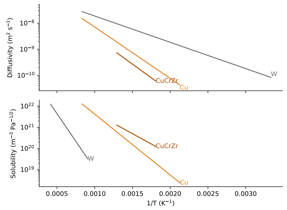
Materials properties
Trapping parameters
| W | |||||
| Cu | |||||
| CuCrZr |
Simulation parameters
Thermal properties
W

14 mm
⌀ 12 mm
1.5 mm
1 mm
Geometry
Cu
CuCrZr

- Maximum 77% difference
- Equivalent trap:
- $$n=n_1 + n_2$$
- $$E_p = \frac{E_{p,1}\ n_1 + E_{p,2} \ n_2}{n} $$

Approximations
Neglecting Trap 2
A 2D model is the best trade-off between performance and accuracy


When neglecting desorption on gaps
3D = 2D
H concentration
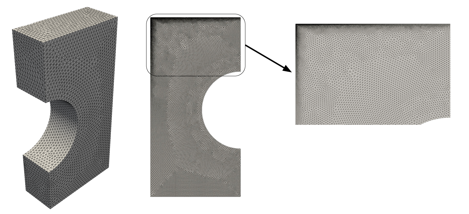
160k tetrahedrons
59k triangles
2D allows for a more refined model
ITER operations will be pulsed

Hot
Cold
The H inventory is influenced by the temperature evolution

Hot
Cold
H inventory (\(\mathrm{m^{-2}}\) )

Assuming a continuous exposure allows to have a bigger stepsize
Cycling: 1500 timesteps
Continuous: 86 timesteps
H inventory (\(\mathrm{m^{-2}}\) )
Low flux:
\( 5.0 \ \mathrm{MW \ m^{-2}} \)
\( 5.0 \times 10^{21}\ \mathrm{m^{-2} \ s^{-1}} \)
High flux:
\( 13 \ \mathrm{MW \ m^{-2}} \)
\( 1.6 \times 10^{22}\ \mathrm{m^{-2} \ s^{-1}} \)
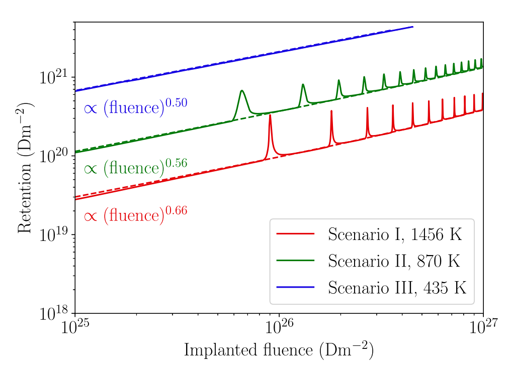
Similar results were obtained with MHIMS
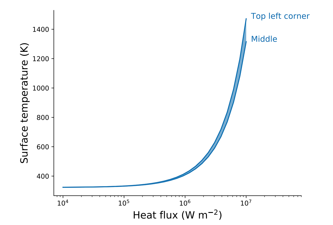
Monoblock thermal response
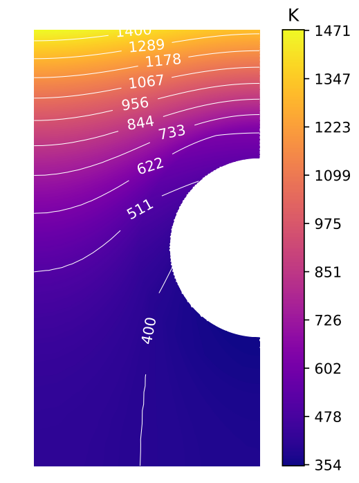
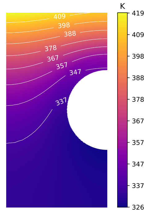
- High temperature gradient
- 2D temperature field
Monoblock thermal response


H concentration
At
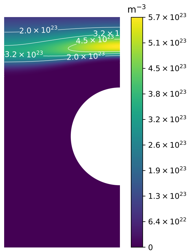
- Penetration front
- High retention zone in colder regions

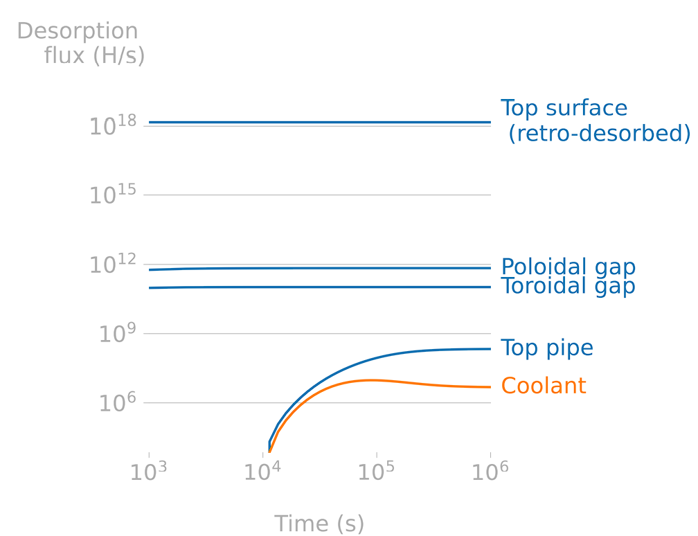
Permeation to coolant
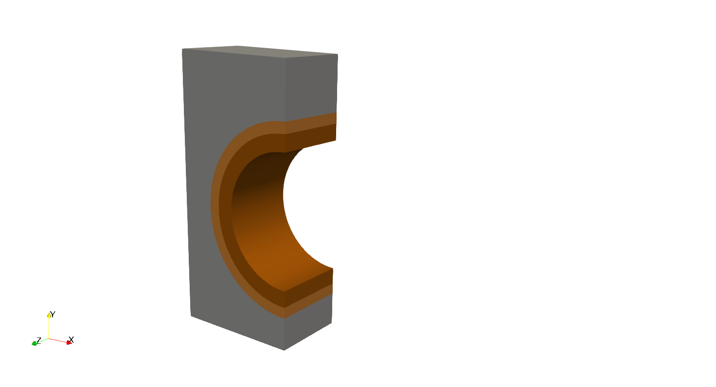
DEMO monoblock
Influence of non-instantaneous recombination


wo gap and wo recombination, independent of thickness (2D)
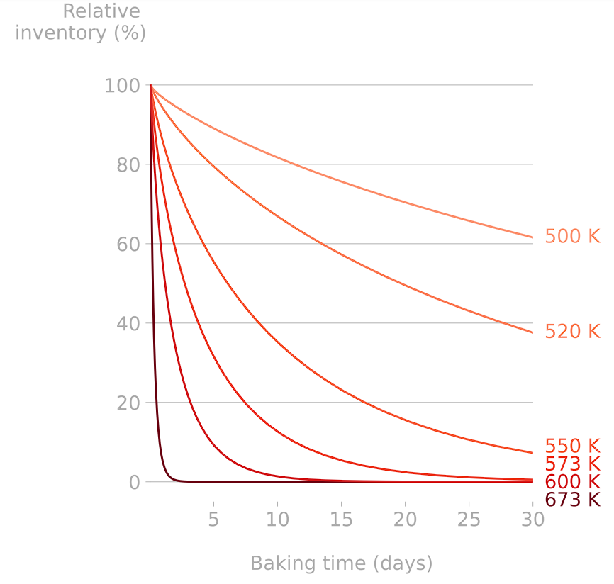
Monoblock baking
To be published
H concentration
At
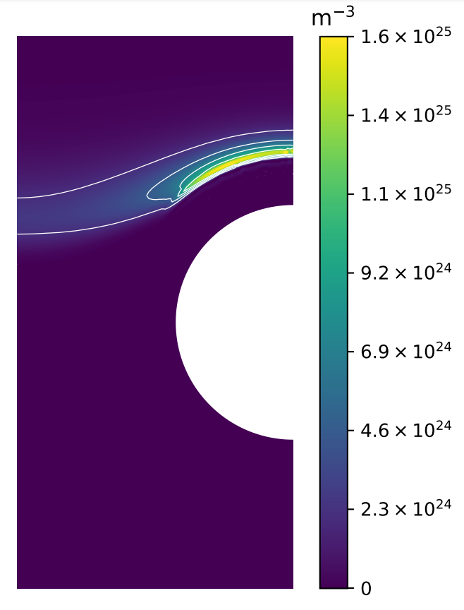

Parametric study


+
+
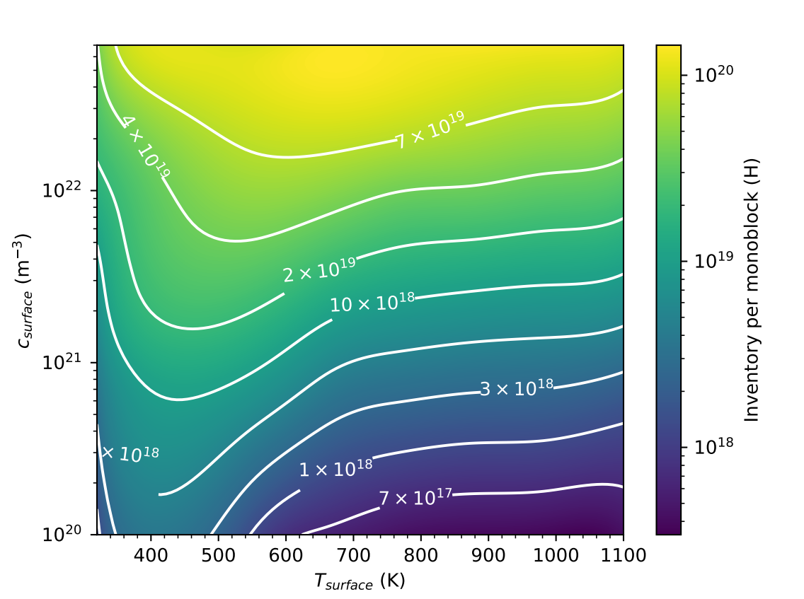
\( T_\mathrm{surface} \) (K)
\( c_\mathrm{surface} \) (\(\mathrm{m}^{-3}\))
Parametric study
+
+

+
+
+
+
+
+
+
+
+
+
+
+
\( T_\mathrm{surface} \) (K)
\( c_\mathrm{surface} \) (\(\mathrm{m}^{-3}\))
Parametric study

At
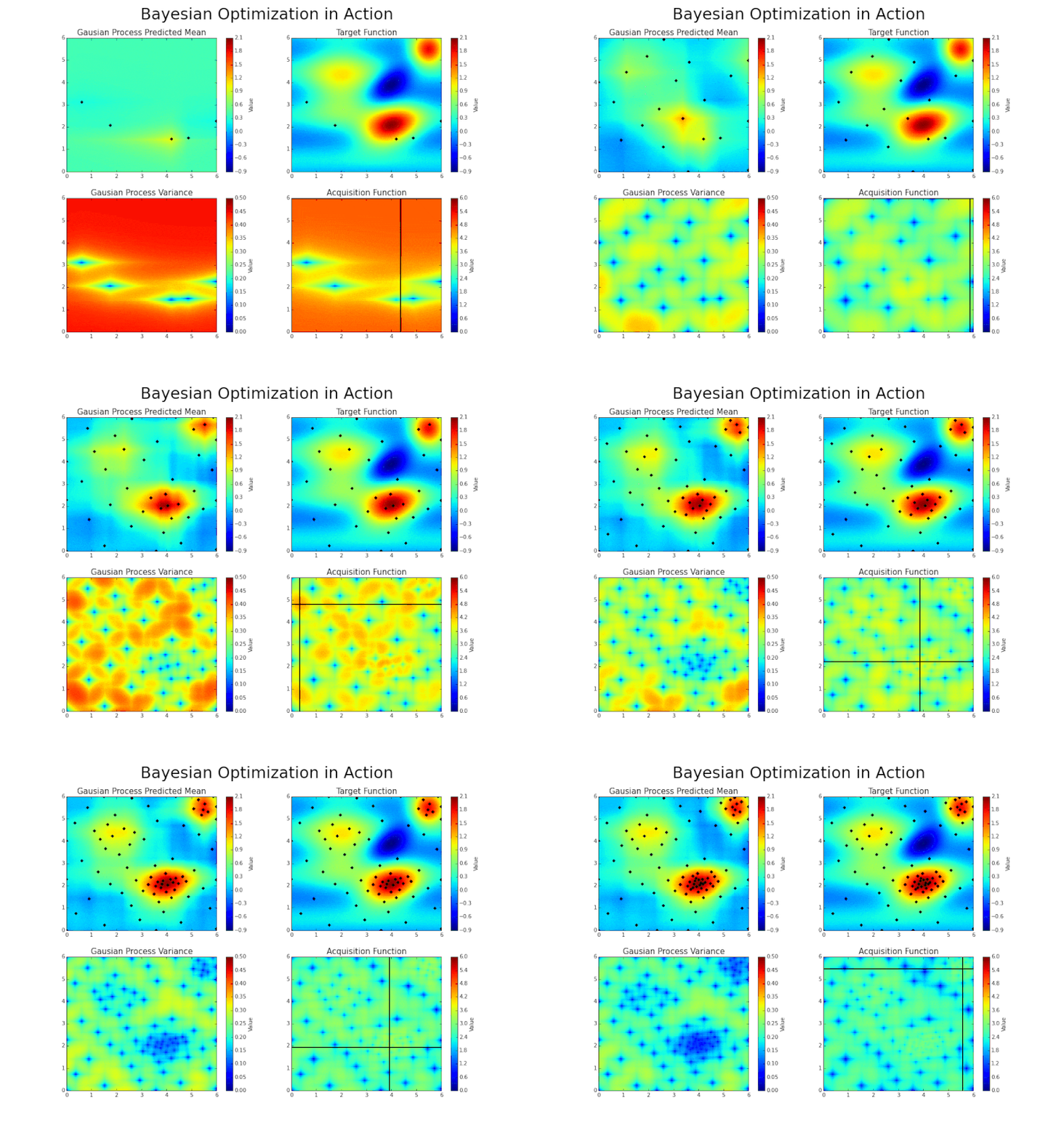
Gaussian Process Regression (GPR)
\( T_\mathrm{surface} \) (K)
\( c_\mathrm{surface} \) (\(\mathrm{m}^{-3}\))
Gaussian process regression
https://juanitorduz.github.io/gaussian_process_reg/
Parametric study

Monoblock behaviour law
At
Rapid assessment of monoblock inventories
\( c_\mathrm{surface} \) (\(\mathrm{m}^{-3}\))
\( T_\mathrm{surface} \) (K)
+
+
+
+
+
+
+
+
+
+
A better behaviour law
Instantaneous recombination
✔️Non homogeneous surface temperature
✔️Non homogeneous surface concentration
❌Only works for instantaneous recombination
+
+
+
+
+
+
+
+
+
+
A better behaviour law
Non-instantaneous recombination
✔️Non homogeneous surface temperature
✔️Non homogeneous surface concentration
✔️Non-instantaneous recombination
❌3 independent variables
+
A better behaviour law
Automatic sampling
Scaling up to the divertor?


Inner Vertical Target
Inner Strike Point
Outer Strike Point
Outer Vertical Target
Dome
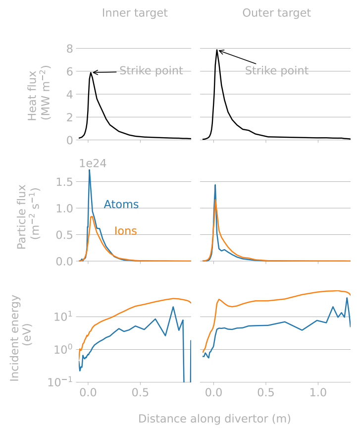
Converting plasma inputs...


Heat flux from SOLPS
Shot #2399
Plasma codes
Mass transport
Momentum
Ions energy \(T_\mathrm{i}\)
Electrons energy \(T_\mathrm{e}\)
\( n \): density
\( u \): velocity
Surface concentration can be estimated
Implantation depth \(R_p\)
Depth
Concentration
$$\varphi_\mathrm{imp}$$
$$\varphi_\mathrm{diff}$$
$$\varphi_\mathrm{desorption}$$
$$\varphi_\mathrm{imp} = \varphi_\mathrm{desorption} + \varphi_\mathrm{diff} $$
When \(\varphi_\mathrm{diff} \ll \varphi_\mathrm{desorption} \rightarrow c_\mathrm{max} = \frac{\varphi_\mathrm{imp} \, R_p }{D}\)
\( c_\mathrm{max}\)

Converting plasma inputs...
Implantation range and reflection coeff. are obtained from SRIM


Use of SRIM is questionable here...

The flux of He is \( \approx \) 1 % of that of D
...to divertor inventory

Monoblock inventory

+
Divertor inventory


Exposure conditions can be obtained for several divertor pressures
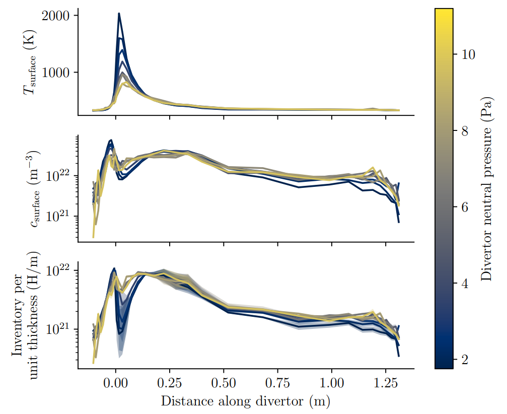
SOLPS runs: Pitts et al NME (2020)

The inventory is estimated from the surrogate model

SOLPS runs: Pitts et al NME (2020)
- The strike point is not the maximum H inventory
- The total divertor inventory can be computed
$$\mathrm{inv}_\mathrm{divertor} = N_\mathrm{cassettes} ( N_\mathrm{PFU-IVT} \int \mathrm{inv}_\mathrm{IVT} (x) dx + $$
$$N_\mathrm{PFU-OVT} \int \mathrm{inv}_\mathrm{OVT} (x) dx )$$
The inventory is estimated from the surrogate model


SOLPS runs: Pitts et al NME (2020)
- The strike point is not the maximum H inventory
- The total divertor inventory can be computed
$$\mathrm{inv}_\mathrm{divertor} = 54 ( 16 \int \mathrm{inv}_\mathrm{IVT} (x) dx + $$
$$22 \int \mathrm{inv}_\mathrm{OVT} (x) dx )$$
The inventory is estimated from the surrogate model
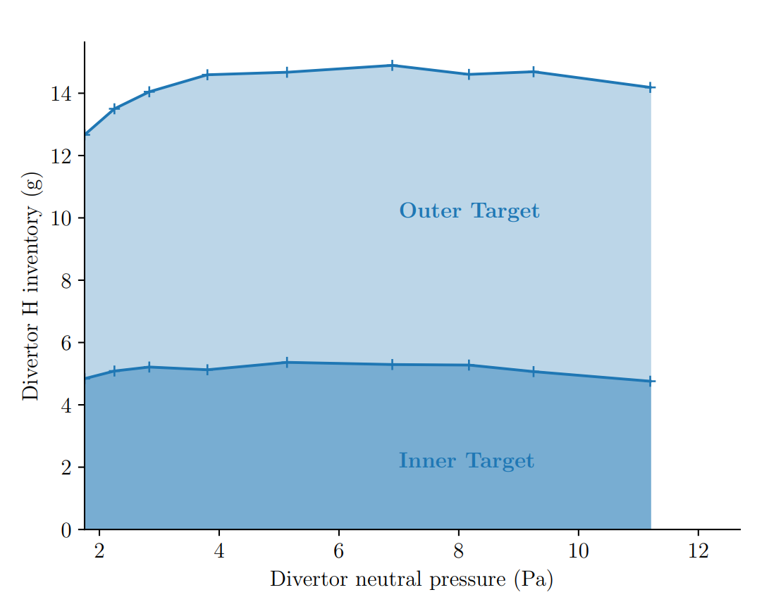
Divertor H inventory (g) at \( t = 10^7 \, \mathrm{s}\)
Safety limit \( = \) 700 g of tritium
\( \max \approx \) 2 % limit ✅

ITER divertor inventory

Safety limit \( = \) 700 g of tritium
\( \max \approx \) 2 % limit ✅
Assuming 50% T
\( \approx \) 1% limit ✅

ITER divertor inventory
Divertor H inventory (g) at \( t = 10^7 \, \mathrm{s}\)
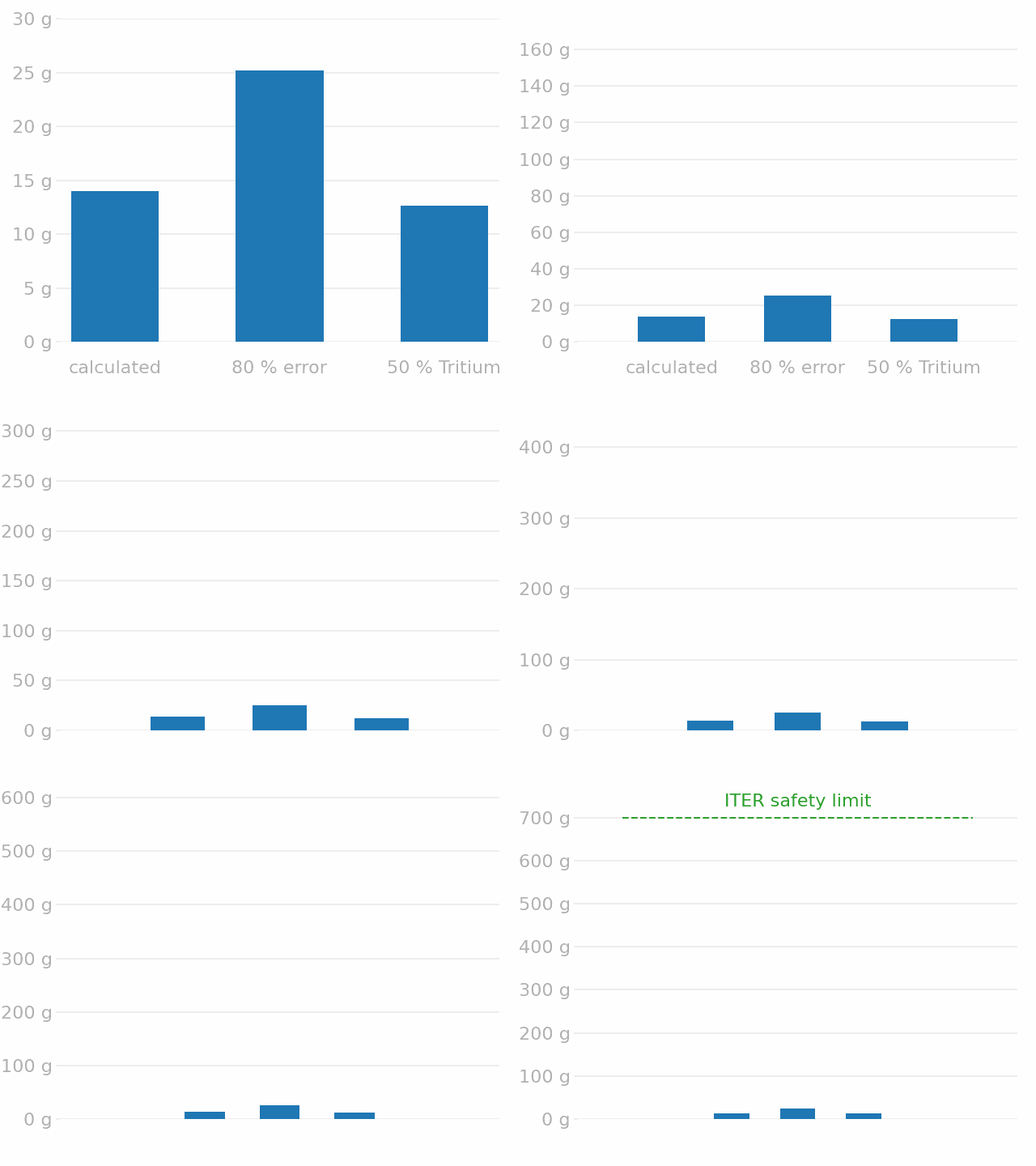
Neglecting trap 2
Influence of helium on hydrogen transport

Why should we care?

Why should we care?
Bubbles


Tungsten fuzz
Thermo-mechanical properties
Tritium production
Hydrogen transport
Sources of helium

Neutronics monoblock simulations with OpenMC
500 MW of fusion power
\(\approx 10^{20} \mathrm{n/s} \)

500 MW of fusion power
\(\approx 10^{20} \mathrm{n/s} \)
Energy released by 1 DT reaction:
\(17.58 \ \mathrm{MeV} = 2.81 \times 10^{-12} \ \mathrm{J}\)
Tally (n,Xa) reaction

DT neutron source energy spectrum

He generation distribution
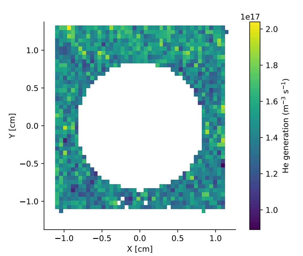
Standard deviation


Neutronic heating
Todo: assess influence of this on the thermals
Sources of helium


Tritium decay simulations with FESTIM
Neutronics monoblock simulations with OpenMC
Tritium decay
Decay constant \( \lambda = 1.77 \times 10^{-9} \ \mathrm{s}^{-1}\)
Decay source for Helium: \( \lambda \sum c_i \)
Sources of helium


Tritium decay simulations with FESTIM
Neutronics monoblock simulations with OpenMC
→ Focus on direct implantation


He\(_1\)
He\(_2\)
He\(_4\)
He\(_3\)
V\(_1\)He\(_7\)
V\(_1\)He\(_8\)
V\(_1\)He\(_9\)
V\(_1\)He\(_{10}\)
Our clustering scheme
Trap mutation
or
self-trapping
\( \frac{\partial c_1}{\partial t} = \nabla \cdot (D_1 \nabla c_1) + P_1 - 2 k^+_{1, 1} c_1^2 - \sum\limits_{i=2}^{6}k_{1,i}^+ c_1 c_i - \langle k_b^+\rangle c_1 c_b \)
$$ \vdots $$
\( \frac{\partial c_6}{\partial t} = \nabla \cdot (D_6 \nabla c_6) - k^+_{1, 6} c_1 c_6 + k_{1,5}^+ c_1 c_{5} \)
\( \frac{\partial c_b}{\partial t} = k_{1,6}^+ c_1 c_{6} \)
\(\frac{\partial \langle i_b \rangle c_b}{\partial t} = 7 k_{1, 6}^+ c_1 c_6 + \langle k_b^+ \rangle c_1 c_b \)
Our clustering scheme
average clustering rate in bubbles
\( \langle k_b^+ \rangle = 4 \pi D_1 (r_1 + \langle r_b \rangle)\)
average bubble radius
\( \langle r_b \rangle = r_{\mathrm{He}_0\mathrm{V}_1} + \left( \frac{3}{4\pi} \frac{a_0^3}{2} \frac{\langle i_b \rangle}{4} \right)^{1/3} - \left( \frac{3}{4\pi} \frac{a_0^3}{2} \right)^{1/3}\)
Only 8 equations:
Let's consider the following reactions
Helium clustering (or emission)
Trap mutation
For each reaction
3-species model:
Rate constants:
N-species model:
Diffusion coefficients
Capture radii
Diffusion
Production
Reaction
Binding energy
Derivation of the forward reaction rate
\(n_i\): local concentration
\(c_i \): mean concentration
\( r_{i,j} = r_i + r_j \): coordinate where the reaction happens (capture radii)

$$c_i$$
$$j$$
in spherical coordinates
2 diffusive species from superpostion principle:
$$k_{i,j}^+ = 4\pi \ r_{i,j} \ (D_i + D_j) $$
Issue #1: Too many equations
\( \frac{\partial c_1}{\partial t} = \nabla \cdot (D_1 \nabla c_1) + P_1 - 2 k^+_{1, 1} c_1^2 - \sum\limits_{i=2}^\infty k_{1,i}^+ c_1 c_i \)
$$ \vdots $$
\( \frac{\partial c_i}{\partial t} = \nabla \cdot (D_i \nabla c_i) - k^+_{1, i} c_1 c_i + k_{1,i-1}^+ c_1 c_{i-1} \)
$$ \vdots $$
\( \frac{\partial c_{N}}{\partial t} =\) \(- k^+_{1, N} c_1 c_{N}\) \( + k_{1,N-1}^+ c_1 c_{N-1} \)
\( \frac{\partial c_{N+1}}{\partial t} =\) \(- k^+_{1, N+1} c_1 c_{N+1}\) \( + k_{1,N}^+ c_1 c_{N} \)
\( \frac{\partial c_{N+2}}{\partial t} =\) \(- k^+_{1, N+2} c_1 c_{N+2}\) \( + k_{1,N+1}^+ c_1 c_{N+1} \)
$$ \vdots $$
💪
\( \frac{\partial c_1}{\partial t} = \nabla \cdot (D_1 \nabla c_1) + P_1 - 2 k^+_{1, 1} c_1^2 - \sum\limits_{i=2}^\infty k_{1,i}^+ c_1 c_i \)
$$ \vdots $$
\( \frac{\partial c_i}{\partial t} = \nabla \cdot (D_i \nabla c_i) - k^+_{1, i} c_1 c_i + k_{1,i-1}^+ c_1 c_{i-1} \)
$$ \vdots $$
\( \frac{\partial c_{N+1}}{\partial t} =\) \(- k^+_{1, N+1} c_1 c_{N+1}\) \( + k_{1,N}^+ c_1 c_{N} \)
\( \frac{\partial c_{N+2}}{\partial t} =\) \(- k^+_{1, N+2} c_1 c_{N+2}\) \( + k_{1,N+1}^+ c_1 c_{N+1} \)
\( \frac{\partial c_{N+3}}{\partial t} =\) \(- k^+_{1, N+3} c_1 c_{N+3}\) \( + k_{1,N+2}^+ c_1 c_{N+2} \)
$$ \vdots $$
💪
Issue #1: Too many equations
\( \frac{\partial c_1}{\partial t} = \nabla \cdot (D_1 \nabla c_1) + P_1 - 2 k^+_{1, 1} c_1^2 - \sum\limits_{i=2}^\infty k_{1,i}^+ c_1 c_i \)
$$ \vdots $$
\( \frac{\partial c_i}{\partial t} = \nabla \cdot (D_i \nabla c_i) - k^+_{1, i} c_1 c_i + k_{1,i-1}^+ c_1 c_{i-1} \)
$$ \vdots $$
\( \sum\limits_{i=N+1}^{\infty} \frac{\partial c_i}{\partial t} = k_{1,N}^+ c_1 c_{N} \)
💪
Issue #1: Too many equations
\( \frac{\partial c_1}{\partial t} = \nabla \cdot (D_1 \nabla c_1) + P_1 - 2 k^+_{1, 1} c_1^2 - \sum\limits_{i=2}^\infty k_{1,i}^+ c_1 c_i \)
$$ \vdots $$
\( \frac{\partial c_i}{\partial t} = \nabla \cdot (D_i \nabla c_i) - k^+_{1, i} c_1 c_i + k_{1,i-1}^+ c_1 c_{i-1} \)
$$ \vdots $$
\( \frac{\partial c_b}{\partial t} = k_{1,N}^+ c_1 c_{N} \)
\( c_b = \sum\limits_{i=N+1}^{\infty} c_i \) : bubble concentration
💪
Issue #1: Too many equations
\( \frac{\partial c_1}{\partial t} = \nabla \cdot (D_1 \nabla c_1) + P_1 - 2 k^+_{1, 1} c_1^2 - \sum\limits_{i=2}^{N}k_{1,i}^+ c_1 c_i - \sum\limits_{i=N+1}^\infty k_{i, 1}^+c_i c_1 \)
$$ \vdots $$
\( \frac{\partial c_i}{\partial t} = \nabla \cdot (D_i \nabla c_i) - k^+_{1, i} c_1 c_i + k_{1,i-1}^+ c_1 c_{i-1} \)
$$ \vdots $$
\( \frac{\partial c_b}{\partial t} = k_{1,N}^+ c_1 c_{N} \)
\( c_b = \sum\limits_{i=N+1}^{\infty} c_i \) : bubble concentration
💪
Issue #1: Too many equations
\( \frac{\partial c_1}{\partial t} = \nabla \cdot (D_1 \nabla c_1) + P_1 - 2 k^+_{1, 1} c_1^2 - \sum\limits_{i=2}^{N}k_{1,i}^+ c_1 c_i - \langle k_b^+\rangle c_1 c_b \)
$$ \vdots $$
\( \frac{\partial c_i}{\partial t} = \nabla \cdot (D_i \nabla c_i) - k^+_{1, i} c_1 c_i + k_{1,i-1}^+ c_1 c_{i-1} \)
$$ \vdots $$
\( \frac{\partial c_b}{\partial t} = k_{1,N}^+ c_1 c_{N} \)
\( c_b = \sum\limits_{i=N+1}^{\infty} c_i \) : bubble concentration
\( \langle k_b^+ \rangle = \left( \sum\limits_{i=N+1}^{\infty} k_ {i, 1}^+ c_i \right) / c_b\) : average clustering rate in bubbles
💪
Issue #1: Too many equations
\( c_b = \sum\limits_{i=N+1}^{\infty} c_i \) : bubble concentration
\( \langle k_b^+ \rangle = \left( \sum\limits_{i=N+1}^{\infty} k_ {i, 1}^+ c_i \right) / c_b\)
\( = \left(\sum\limits_{i=N+1}^{\infty} 4 \pi D_1 (r_1 + r_i) c_i\right) / c_b \)
💪
average clustering rate in bubbles
Issue #2: what's the value of \( \langle k_b^+ \rangle \)?
Issue #2: what's the value of \( \langle k_b^+ \rangle \)?
\( c_b = \sum\limits_{i=N+1}^{\infty} c_i \) : bubble concentration
\( \langle r_b \rangle = \left( \sum\limits_{i=N+1}^{\infty} r_ i c_i \right) / c_b\) : average bubble radius
\( \langle k_b^+ \rangle \)\( = \left( \sum\limits_{i=N+1}^{\infty} k_ {i, 1}^+ c_i \right) / c_b\)
\( = \left(\sum\limits_{i=N+1}^{\infty} 4 \pi D_1 (r_1 + r_i) c_i\right) / c_b \)
\( =4 \pi D_1 (r_1 + \langle r_b \rangle)\)
💪
average clustering rate in bubbles
\( r_i = r_{\mathrm{He}_0\mathrm{V}_1} + \left( \frac{3}{4\pi} \frac{a_0^3}{2} n_{\mathrm{V},i} \right)^{1/3} - \left( \frac{3}{4\pi} \frac{a_0^3}{2} \right)^{1/3}\)
💪
\( c_b = \sum\limits_{i=N+1}^{\infty} c_i \) : bubble concentration
\( \langle k_b^+ \rangle = 4 \pi D_1 (r_1 + \langle r_b \rangle)\) : average clustering rate in bubbles
\( \langle r_b \rangle = \left( \sum\limits_{i=N+1}^{\infty} r_ i c_i \right) / c_b\) : average bubble radius
Issue #3: what's the value of \( \langle r_b \rangle \)?
\( r_i = r_{\mathrm{He}_0\mathrm{V}_1} + \left( \frac{3}{4\pi} \frac{a_0^3}{2} \frac{i}{4} \right)^{1/3} - \left( \frac{3}{4\pi} \frac{a_0^3}{2} \right)^{1/3}\)
\( n_{\mathrm{V},i} = i/4 \) : 4 He per vacancy
💪
\( c_b = \sum\limits_{i=N+1}^{\infty} c_i \) : bubble concentration
\( \langle k_b^+ \rangle = 4 \pi D_1 (r_1 + \langle r_b \rangle)\) : average clustering rate in bubbles
\( \langle r_b \rangle = \left( \sum\limits_{i=N+1}^{\infty} r_ i c_i \right) / c_b\) : average bubble radius
Issue #3: what's the value of \( \langle r_b \rangle \)?
\( c_b = \sum\limits_{i=N+1}^{\infty} c_i \) : bubble concentration
\( \langle k_b^+ \rangle = 4 \pi D_1 (r_1 + \langle r_b \rangle)\) : average clustering rate in bubbles
\( \langle r_b \rangle = \left( \sum\limits_{i=N+1}^{\infty} r_ i c_i \right) / c_b\) : average bubble radius
\( \langle i_b \rangle = \left( \sum\limits_{i=N+1}^{\infty} i c_i \right) / c_b\) : average He content in bubbles
\( n_{\mathrm{V},i} = i/4 \) : 4 He per vacancy
💪
\( \langle r_b \rangle = r_{\mathrm{He}_0\mathrm{V}_1} + \left( \frac{3}{4\pi} \frac{a_0^3}{2} \frac{\langle i_b \rangle}{4} \right)^{1/3} - \left( \frac{3}{4\pi} \frac{a_0^3}{2} \right)^{1/3}\)
\( r_i = r_{\mathrm{He}_0\mathrm{V}_1} + \left( \frac{3}{4\pi} \frac{a_0^3}{2} \frac{i}{4} \right)^{1/3} - \left( \frac{3}{4\pi} \frac{a_0^3}{2} \right)^{1/3}\)
Issue #3: what's the value of \( \langle r_b \rangle \)?

\( \langle r_b \rangle = r_{\mathrm{He}_0\mathrm{V}_1} + \left( \frac{3}{4\pi} \frac{a_0^3}{2} \frac{\langle i_b \rangle}{4} \right)^{1/3} - \left( \frac{3}{4\pi} \frac{a_0^3}{2} \right)^{1/3}\)
\( \frac{\sum\limits_{i=N+1}^{\infty} i^{1/3} c_i } { c_b} \approx \left( \sum\limits_{i=N+1}^{\infty} i c_i / c_b \right)^{1/3} = \langle i_b \rangle ^{1/3}\)
When \( c_i \) has a narrow gaussian distribution (ie. \(\sigma / \mu \ll 1\) )
Sum approximation
\( \langle i_b \rangle = \left( \sum\limits_{i=N+1}^{\infty} i c_i \right) / c_b\)
\( \langle i_b \rangle c_b= \sum\limits_{i=N+1}^{\infty} i c_i \)
\(\frac{\partial \langle i_b \rangle c_b}{\partial t} = \sum\limits_{i=N+1}^{\infty} i \frac{\partial c_i}{\partial t}\)
💪
\(\frac{\partial \langle i_b \rangle c_b}{\partial t} = (N+1) k_{1, N}^+ c_1 c_N + \langle k_b^+ \rangle c_1 c_b \)
↓ trust me
\( c_b = \sum\limits_{i=N+1}^{\infty} c_i \) : bubble concentration
\( \langle k_b^+ \rangle = 4 \pi D_1 (r_1 + \langle r_b \rangle)\) : average clustering rate in bubbles
\( \langle i_b \rangle = \left( \sum\limits_{i=N+1}^{\infty} i c_i \right) / c_b\) : average He content in bubbles
Issue #4: what's the value of \( \langle i_b \rangle \)?
\( \frac{\partial c_1}{\partial t} = \nabla \cdot (D_1 \nabla c_1) + P_1 - 2 k^+_{1, 1} c_1^2 - \sum\limits_{i=2}^{N-1}k_{1,i}^+ c_1 c_i - \langle k_b^+\rangle c_1 c_b \)
$$ \vdots $$
\( \frac{\partial c_i}{\partial t} = \nabla \cdot (D_i \nabla c_i) - k^+_{1, i} c_1 c_i + k_{1,i-1}^+ c_1 c_{i-1} \)
$$ \vdots $$
\( \frac{\partial c_b}{\partial t} = k_{1,N}^+ c_1 c_{N} \)
💪
\(\frac{\partial \langle i_b \rangle c_b}{\partial t} = (N+1) k_{1, N}^+ c_1 c_N + \langle k_b^+ \rangle c_1 c_b \)
\( c_b = \sum\limits_{i=N+1}^{\infty} c_i \) : bubble concentration
\( \langle k_b^+ \rangle = 4 \pi D_1 (r_1 + \langle r_b \rangle)\) : average clustering rate in bubbles
\( \langle i_b \rangle = \left( \sum\limits_{i=N+1}^{\infty} i c_i \right) / c_b\) : average He content in bubbles
Issue #4: what's the value of \( \langle i_b \rangle \)?
Assumption time!
- Only pure He clusters are mobile
- Trap-mutation from 7 He
- Grouping starts at \( i > 6 \)
- He/V ratio: 4
- No He emission from bubbles
- Pre-existing vacancies are neglected
- We don't solve for W self-interstitials
-
Diffusion coefficients from Faney et al. Nucl. Fusion (2015)
-
Dissociation energies from Becquart et al. J. Nucl. Mater. (2010)
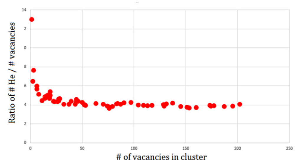
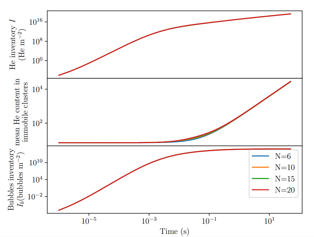
Varying the grouping threshold
Results on a half-slab case

- Helium first diffuses rapidly into the bulk
- Mobile helium is consumed to form bubbles
\(c_i = 0 \)
W
He implantation
Mobile helium
Bubbles
Retention
$$\mathrm{m}^{-3}$$
Half-slab case
- "Semi-infinite" (0.6 mm)
-
Helium source
- 100 eV
-
Gaussian distribution
- \( \mu =1.5 \mathrm{nm} \, \sigma = 1.5 \mathrm{nm} \)
- Flux \( 10^{22} \, \mathrm{m^{-2} \, s^{-1} }\)
- Temperature 1000 K
\(c_i = 0 \)
0.6 mm
Code comparison

Faney et al. Nucl. Fusion 2014
- 100 eV He
- Flux \( 10^{22} \mathrm{\, m^{-2} \, s^{-1}} \)
- Fluence \(5 \times 10^{25} \mathrm{\ m^{-2}} \)
30 nm
\( c_i = 0 \)
\( c_i = 0 \)
Discrepancies at high T due to different sets of dissociation energies

Dissociation energy sensitivity
Solid: +0
Dashed: + 0.5 eV
Dash-point: - 0.5 eV
Varying flux and temperature

\( c_\mathrm{He_1 \, ideal} = \frac{\varphi_\mathrm{imp} R_p}{D_1(T)} \)
Varying temperature and particle flux
Parametric study


1 h
\( \int c_b \langle i_b \rangle dx\)
He inventory in bubbles
Parametric study


1 h
\( \bar{\langle i_b \rangle} = \frac{\int c_b \langle i_b \rangle dx}{\int c_b dx} = \frac{\mathrm{inventory}}{\mathrm{total \, bubbles}}\)
Mean helium content in bubbles
Parametric study
\(\int c_b dx\)
Total bubbles


1 h efef
Two regimes can be identified


Nucleation
🡺Self trapping
🡺\( c_b \) increases
Growth
🡺\( \langle i_b \rangle \) increases
🡺\( \langle k_b^+ \rangle \) increases
\( \langle i_b \rangle \) is low
\( \langle k_b^+ \rangle \) is low
When \( c_b \) is large enough
Two regimes can be identified

\(\frac{\partial c_b}{\partial t} = k_{1, N}^+ c_1 c_N\)
\(\frac{\partial \langle i_b \rangle c_b}{\partial t} = (N+1) k_{1, N}^+ c_1 c_N + \langle k_b^+ \rangle c_1 c_b \)
\( \langle i_b \rangle \approx 7 \Leftrightarrow \langle k_b^+ \rangle \approx 0\)
\( \Leftrightarrow \frac{\partial \langle i_b \rangle c_b}{\partial t} \approx (N+1) k_{1, N}^+ c_1 c_N \)
\( \Leftrightarrow \langle i_b \rangle \frac{\partial c_b}{\partial t} + c_b \frac{\partial \langle i_b \rangle}{\partial t} \approx (N+1) k_{1, N}^+ c_1 c_N \)
\( \Leftrightarrow \frac{\partial \langle i_b \rangle}{\partial t} \propto N +1 - \langle i_b \rangle \approx 0\)
\( c_b \gg c_N \)
\(\Leftrightarrow c_N \approx 0 \)
\(\Leftrightarrow \frac{\partial c_b}{\partial t} \approx 0 \)
\( \Leftrightarrow \frac{\partial \langle i_b \rangle c_b}{\partial t} \approx \langle k_b^+ \rangle c_1 c_b \)
\( \Leftrightarrow \frac{\partial \langle i_b \rangle}{\partial t} \approx \langle k_b^+ \rangle c_1\)
Nucleation regime
Growth regime

N cannot be lower than 6
Regime where intermediate clusters don't matter anymore
The bubble growth model was compared with experiments

Mykola Ialovega's PhD research

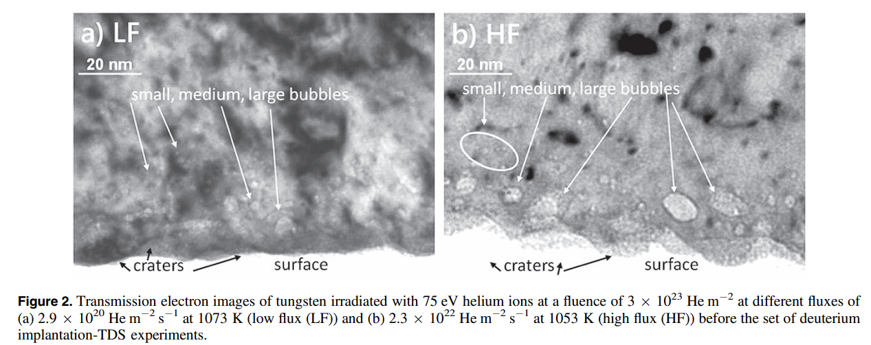
\(75 \ \mathrm{eV}\) He at \( 2.3 \times 10^ {22} \ \mathrm{m^{-2} \ s^{-1}}\) and \(1053 \ \mathrm{K} \) for \(13 \ \mathrm{s}\)
How to couple this to H transport?
Ialovega's experiment
He exposure
D exposure
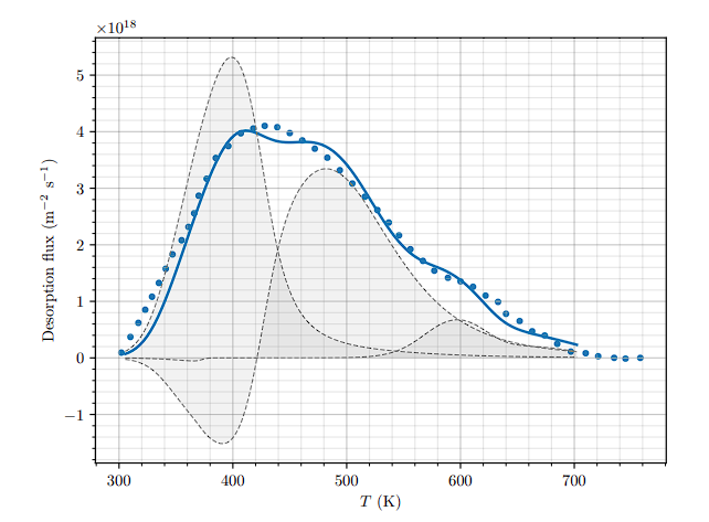
Thermo-desorption
Repeat 5 times
W
Experimental conditions
Sample: \(100 \ \mathrm{\mu m} \) W
Pre-damage: \(75 \ \mathrm{eV}\) He at \( 2.3 \times 10^ {22} \ \mathrm{m^{-2} \ s^{-1}}\) and \(1053 \ \mathrm{K} \) for \(13 \ \mathrm{s}\)
Initial cleaning TDS after He implantation up to 870 K
D exposure: 250 eV at room temperature
Flux: \( 1.7 \times 10^ {16} \ \mathrm{m^{-2} \ s^{-1}}\)
Fluence: \( 4.5 \times 10^ {19} \ \mathrm{m^{-2}}\)
TDS temperature ramp: 1 K/s
Ialovega's experiment
Ialovega's experiment

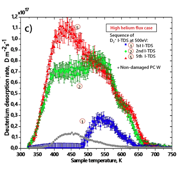
Lack of control experiment
❌No initial TDS
❌No cycling
❌Not performed at the time of the experiment
→ Can only be compared qualitatively!
Ialovega's experiment


Ialovega's experiment


Ialovega's experiment
Correlation He release/D release
Hypotheses
- Helium doesn't desorb from bubbles
- Pre-existing defects exist (suggested by further analysis)
- Helium can saturate traps for Deuterium
surface coverage of trapping sites (tuning parameter)
bubbles radius
bubbles area

The He model was weakly coupled to FESTIM
The model reproduced the experiment

Bubble-induced trap
- 4 traps including a bubble-induced trap
- TDS 1: density of available pre-existing traps is zero
- TDS 2-5: density of pre-existing traps \( \approx 2\times10^{-3}\ \mathrm{at.fr.}\)
- \( f \) is unchanged \( 3 \times 10^{18} \ \mathrm{m^{-2}}\)


Initial state

Pre-existing defects
He implantation

He implantation

1st D implantation


1st D implantation
1st TDS

He is removed from pre-existing defects
D is desorbed from bubbles


2nd D implantation

2nd D implantation

2nd D implantation

2nd TDS

D desorption from secondary defects

Repeat...

Impact on divertor inventory?

Divertor H inventory (g) at \( t = 10^7 \, \mathrm{s}\)
Increased trapping (bubbles)
Reduced trapping
(trap saturation)

Divertor inventory could be even lower
Main conclusions
- FESTIM was developed to assess T inventory in ITER plasma facing components and is now used for other applications (breeding blankets, experimental work...).
- Under conservative assumptions, the T inventory in the ITER divertor is below 1% of the in-vessel safety limit after 25 000 pulses.
- Results suggest that the presence of helium could reduce this inventory further by saturating traps.
Where to go from here?
- Validate the monoblock model with experimental data
- Retention in Be co-deposited layers will domitate the inventory
- Confirm/infirm our interpretation of the He-H interactions
- Investigate other in-vessel components like breeding blankets
Adding bubble bursting


