Introduction: tritium in fusion
22.016
9-18-2025
Remi Delaporte-Mathurin
Introuction - Remi Delaporte-Mathurin
- 2022-today: Researcher at the Plasma Science and Fusion Center, MIT
-
2018-2019: Ph.D. French Atomic Energy Authority (CEA Cadarache) and University Sorbonne Paris Nord
-
2017: CEA Cadarache, IRFM, apprentice
- 2016: UK Atomic Energy Authority
- 2012-2018: M.Sc. Thermal Engineering and Energy Sciences
Joint European Torus (JET), Culham, UK
Introuction - Remi Delaporte-Mathurin
LIBRA tritium breeding experiment
Tritium contamination in a heat exchanger with FESTIM
Hydrogen gas-driven permeation experiment
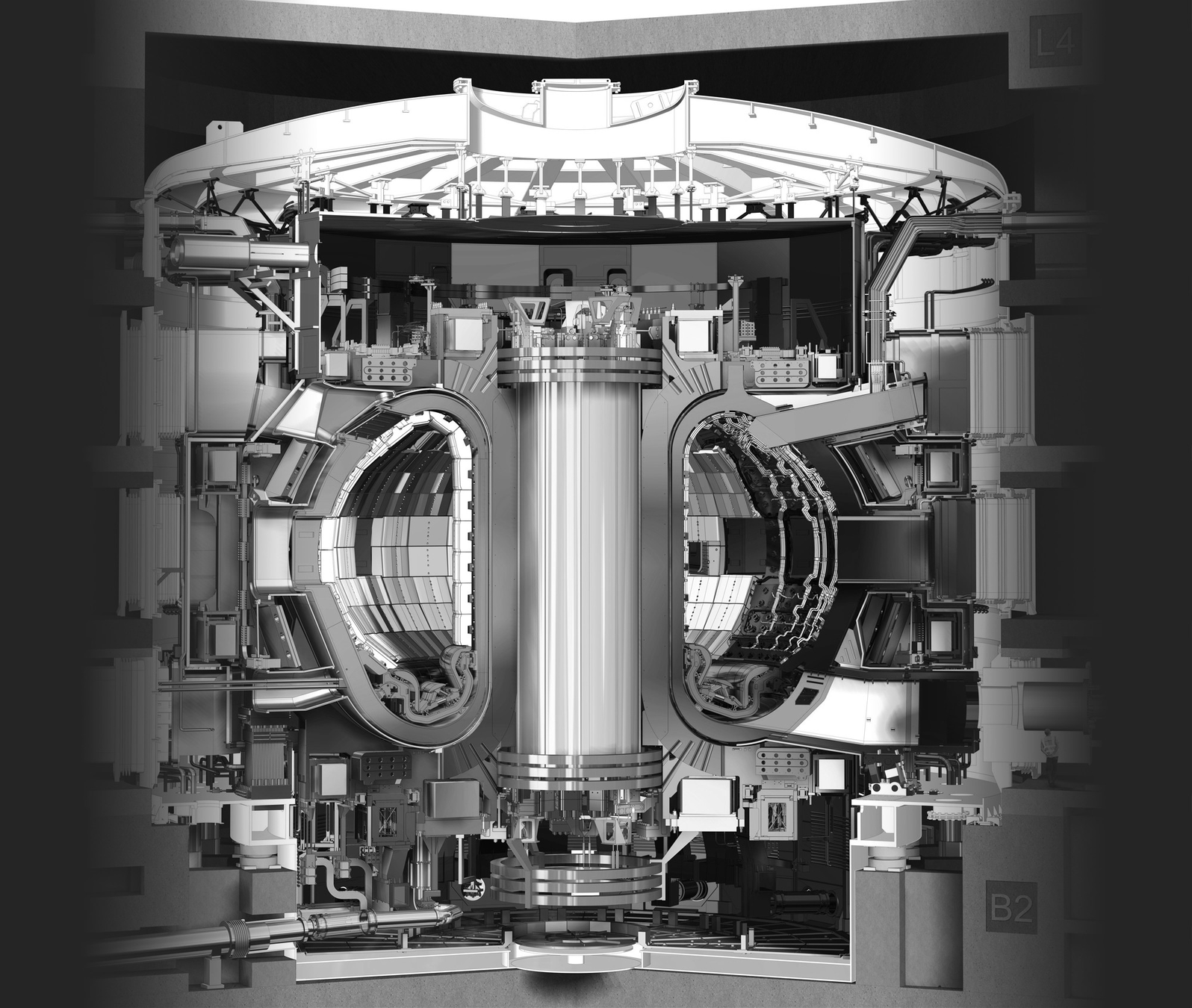
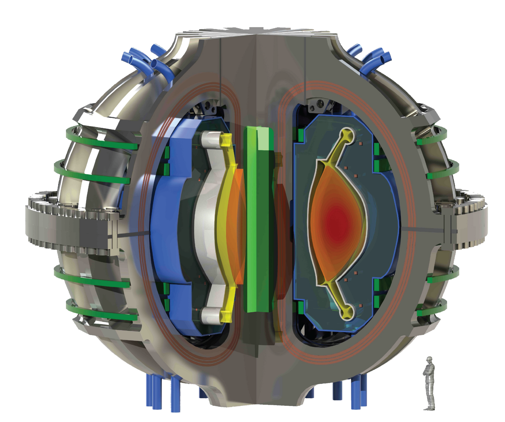
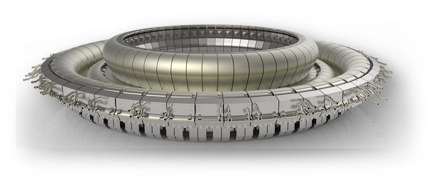
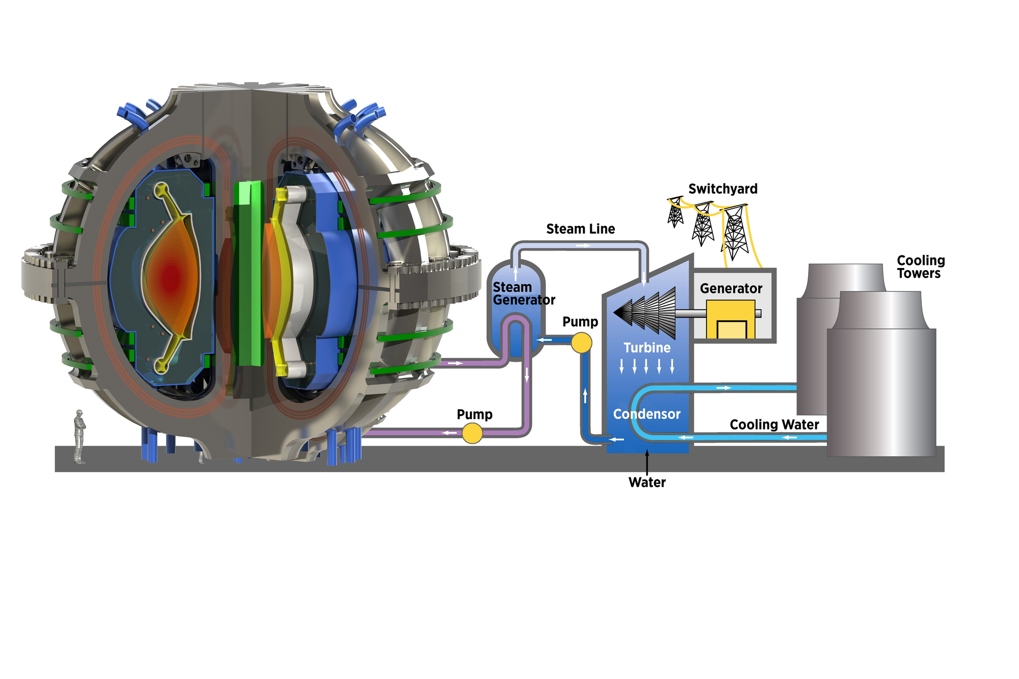
ITER
Plasma: mixture of Hydrogen (D-T) and Helium
Particle bombardment
Divertor
Why should we care?
T is rare
T is expensive
€£$
Material embrittlement
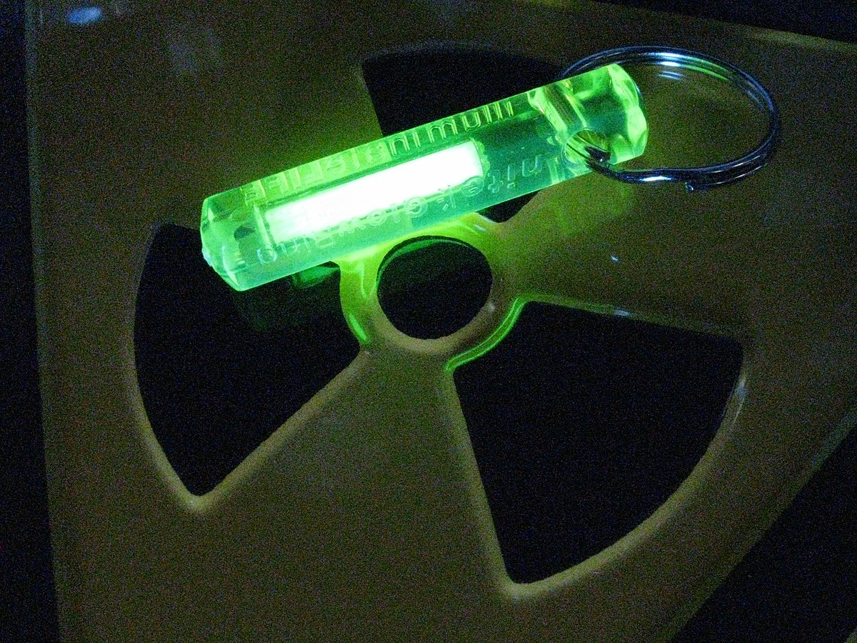
T is radioactive
☢
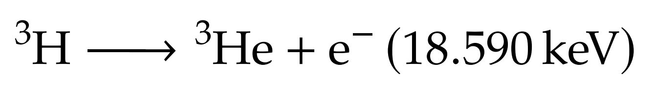
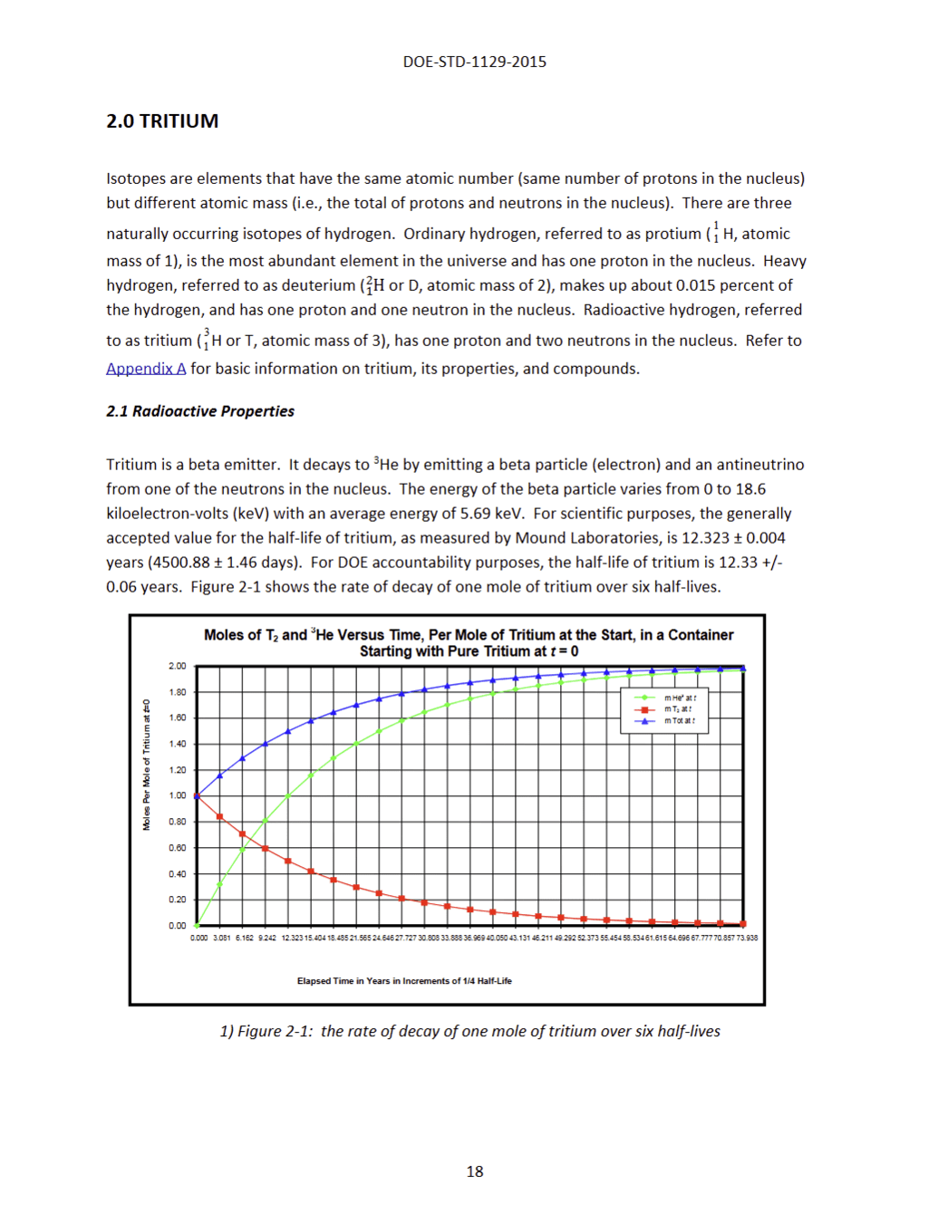
What's Tritium?
+
+
+
Protium
Deuterium
Tritium
Molar mass: 6.032 g/mol
What's Tritium?
+
Tritium
☢
Fuel self-sufficiency

Half-life: 12 years
☢
Consumption of a 1 GWth fusion reactor (1 year)
50 kg
Cost: $30,000 per gram
The breeding blanket
Lithium is used to breed tritium
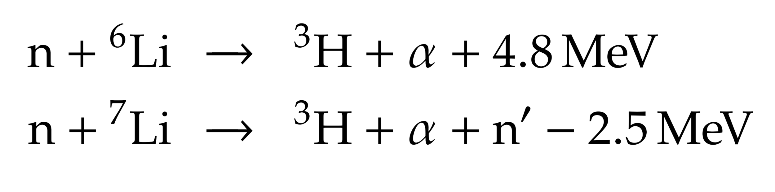
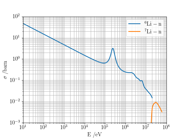
→ Li6 enrichment is an option
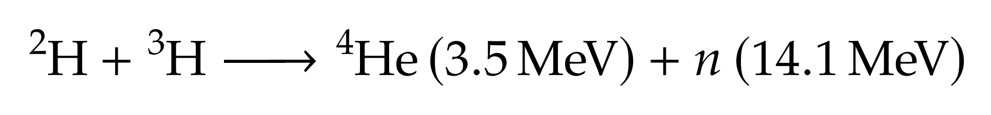
DT fusion neutrons

Magnet
Breeding blanket
The breeding blanket
Plasma
The breeding blanket is only one component of the fuel cycle
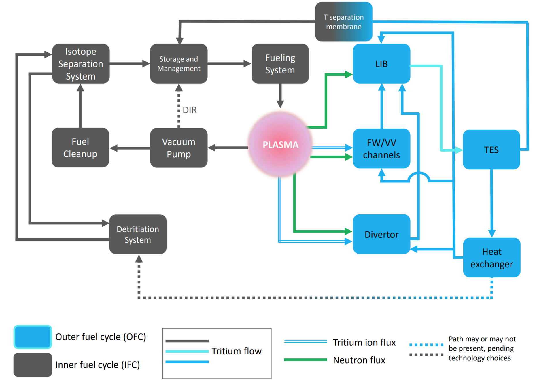
Let's play with a simple fuel cycle model
Burns tritium
Breeds tritium (TBR)
Tritium Extraction System
Breeding Blanket
Plasma
Storage
neutrons
TBR
(constrained by technology)
Doubling time
(driven by economics)
Startup inventory
(constrained by safety)
Startup inventory
Tritium Extraction System
Breeding Blanket
Plasma
Storage
Safety issues
Tritium is a health hazard
☢
- No external hazard: electron stopped by skin
- Once ingested, can cause damage to internal tissues
- Forms: HT, HTO, methane, titrides...
- Biological half-life of HTO: 10 days
- Biological half-life of OBT (Organically Bound Tritium): 40 days
Augustin Janssens. ‘Emerging Issues on Tritium and Low Energy Beta Emitters”’. en. In: (Nov. 2007), p. 100
| Country | Water limit (Bq/L) |
|---|---|
| EU | 100 |
| USA | 740 |
| UK | 100 |
| Canada | 7,000 |
| Finland | 30,000 |
| Australia | 76,103 |
| Russia | 7,700 |
| WHO | 10,000 |
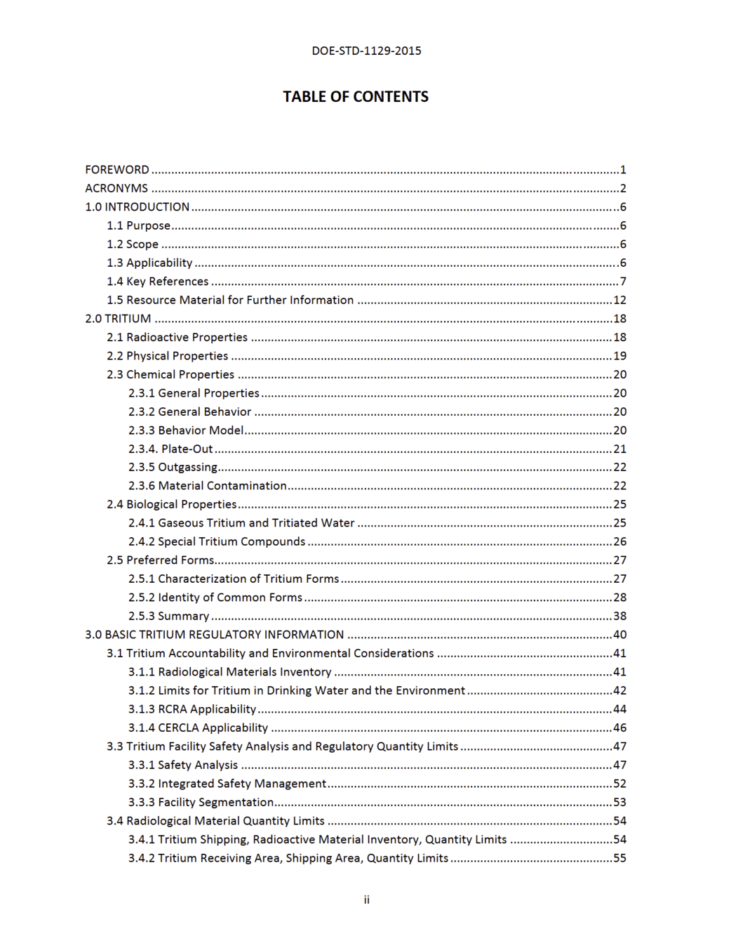
Tritium US DOE Handbook
413 pages!
The tritium content needs to be limited
1. Keep inventory at a minimum
Tritium limit in the ITER vacuum vessel: 1 kg
1. Keep inventory at a minimum
2. Reduce inventory
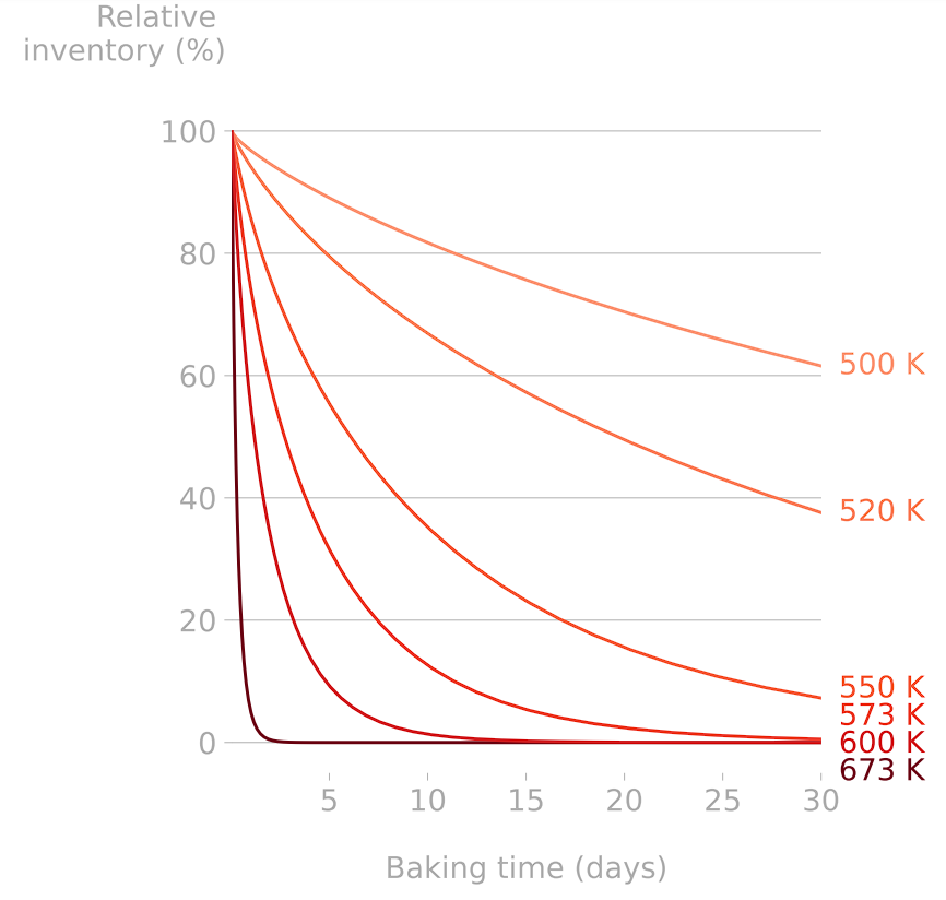
Heating components help releasing their tritium content (cf. Basics of H transport)
The tritium content needs to be limited
1. Keep inventory at a minimum
2. Reduce inventory
3. Avoid contamination of coolants
Metal
Tritiated environment
"Clean" environment
Permeation
The tritium content needs to be limited
1. Keep inventory at a minimum
2. Reduce inventory
3. Avoid contamination of coolants
Metal
Tritiated environment
"Clean" environment
Permeation barrier
Permeation
The tritium content needs to be limited
1. Keep inventory at a minimum
2. Reduce inventory
3. Avoid contamination of coolants
Ceramics are promising candidates:
- oxides
- carbides
- nitrides
Permeation barriers are caracterised by their PRF (Permeation Reduction Factor)
Target for breeding blankets PRF ≈ 100-1000
Luo et al Surface and Coatings Technology 2020
The tritium content needs to be limited
Component embrittlement
Agglomeration of hydrogen can lead to blistering
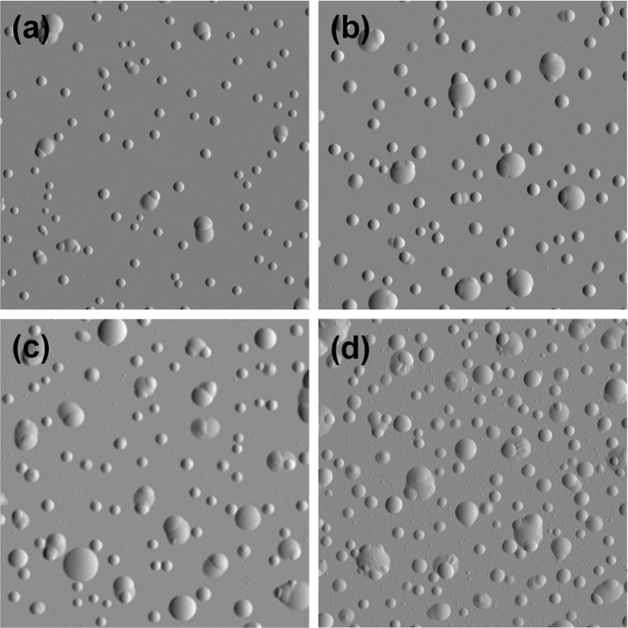
- Accumulation of H at defects:
- Voids
- Reaction with impurities (formation of methane)
- grain boundaries
- Creation of a filled cavity
- Growth of the cavity without bursting
Kuznetsov, Alexey S. et al. “Hydrogen-induced blistering of Mo/Si multilayers: Uptake and distribution.” Thin Solid Films 545 (2013): 571-579.
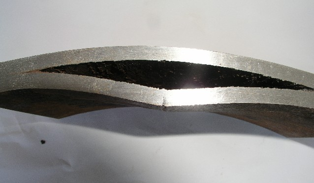
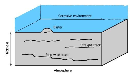
Cavities can lead to Hydrogen Induced Cracking
Review of HIC by Sofronis
https://doi.org/10.1016/j.jngse.2022.104547
Take aways
H transport
Safety
Fusion Economy
Materials
- Minimising inventories
- Limiting permeation
- Protecting personel
- Fuel cycle
- Tritium breeding
- Losses
- Embrittlement
- H induced cracks
DFT
Multi-scale hydrogen transport
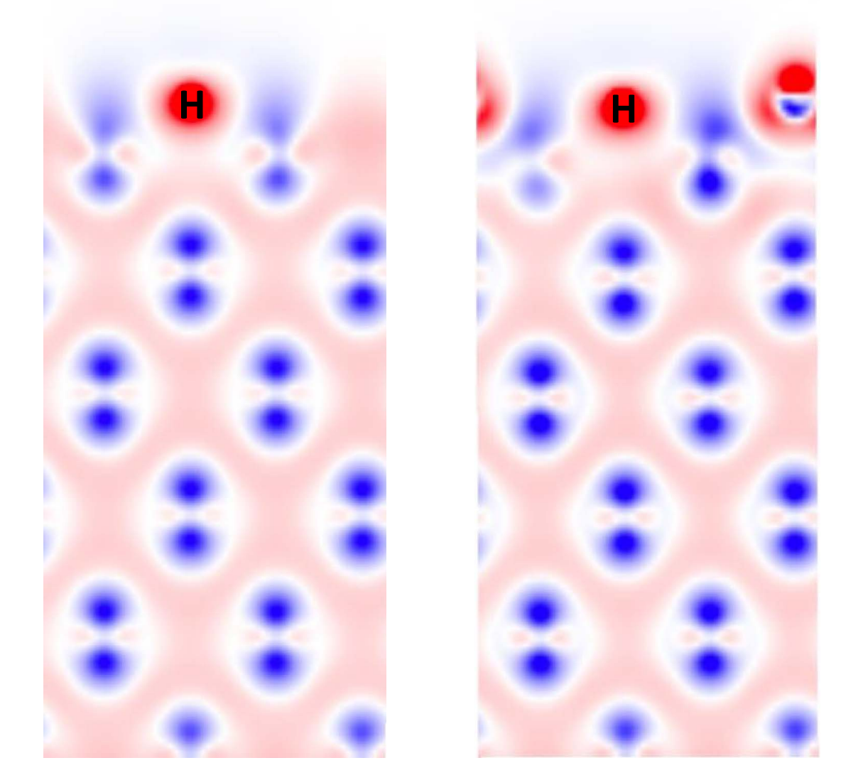
Y. Ferro et al 2023 Nucl. Fusion 63 036017
Length scale
Time scale
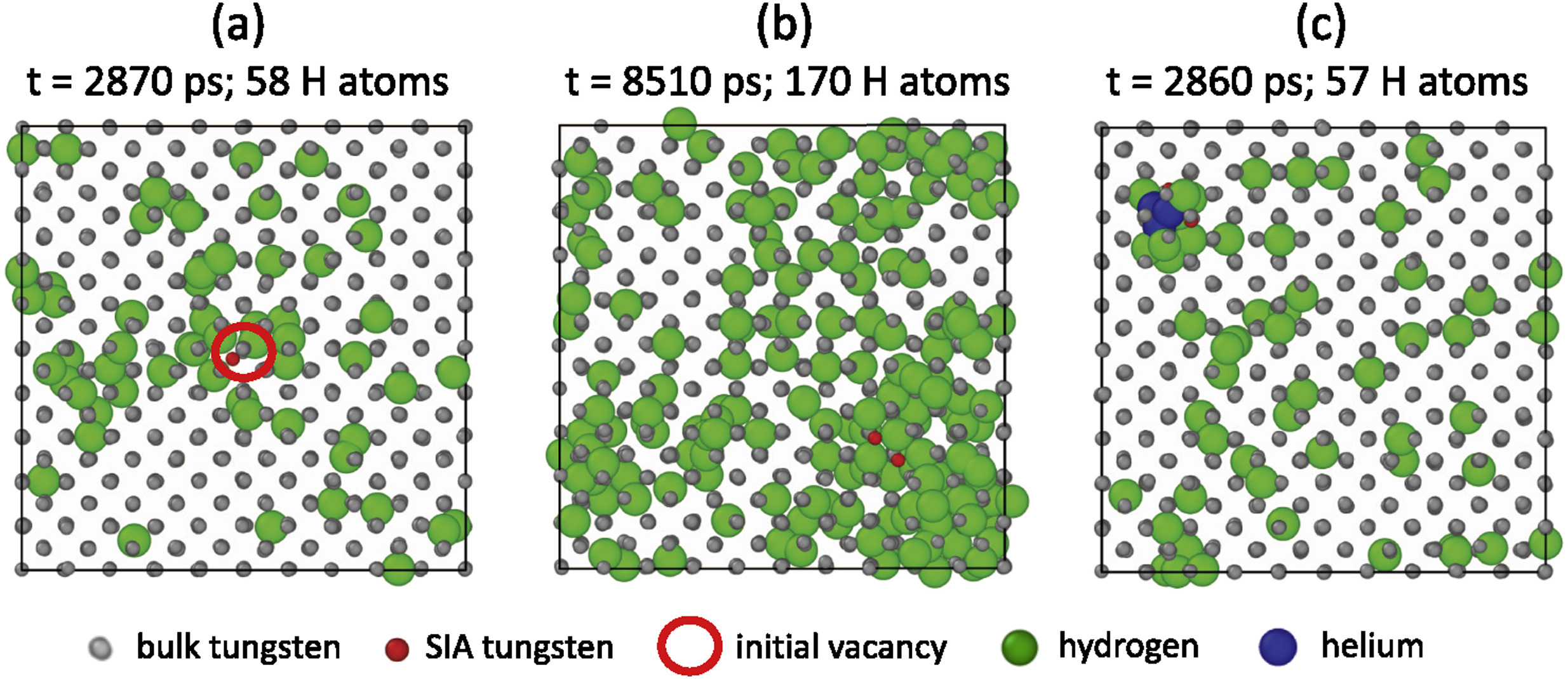
MD
Length scale
Time scale
DFT
potentials
Multi-scale hydrogen transport
Component scale modelling
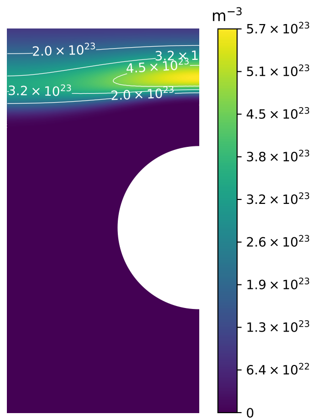
Length scale
Time scale
MD
DFT
D, S, other coeffs.
Multi-scale hydrogen transport
Length scale
Time scale
MD
DFT
Component scale modelling
Fuel cycle modelling
Residency times, fluxes, ...
Multi-scale hydrogen transport
Length scale
Time scale
MD
DFT
Component scale modelling
Fuel cycle modelling
Abstraction
Multi-scale hydrogen transport
Tritium transport theory

Hydrogen transport in metals
Diffusion
Even more particles
continuity approximation
Single particle
Random walk
Many particles
Diffusion
\( \varphi \): diffusion flux
\( D \): diffusion coefficient
\( c \): mobile hydrogen concentration
Fick's 1st law of diffusion
Diffusion
\( \varphi\): diffusion flux
\( D \): diffusion coefficient
\( c \): mobile hydrogen concentration
\( S\): source term
Fick's 1st law of diffusion
Fick's 2nd law of diffusion
Diffusion
\( \varphi\): diffusion flux
\( D \): diffusion coefficient
\( c \): mobile hydrogen concentration
\( S\): source term
Soret effect (or thermophoresis)
Stress assisted diffusion
Particle implantation
Ziegler et al. 2010. Nuclear Instruments and Methods in Physics Research Section B: Beam Interactions with Materials and Atoms, 268 (11): 1818–23. https://doi.org/10.1016/j.nimb.2010.02.091.
Implantation range
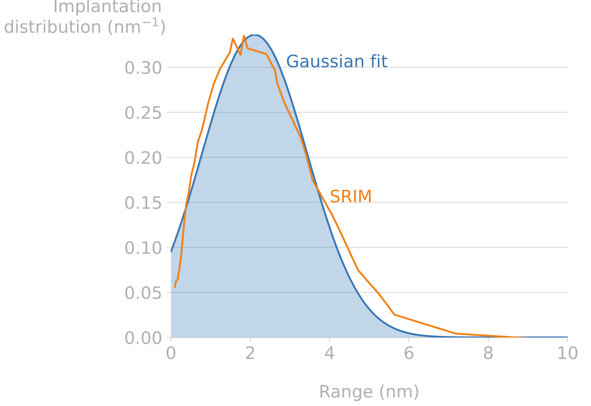
Implantation range & width and reflection coefficient can be computed with SRIM, SDTRIM...
Mutzke et al, SDTrimSP Version 6.00 2019
Particle implantation
\(\Gamma_\mathrm{incident} \): incident flux (particle/m2/s)
\( f(x) \): Gaussian distribution (/m)
\(r \): reflection coefficient
Surface effects
H2 molecules
Metal lattice
Surface effects
Dissociation coefficient (H/m2/s/Pa)
Partial pressure of H (Pa)
Adsorbed H
Metal lattice
Surface effects
Metal lattice
Recombination coefficient (m4/s)
Concentration (H/m3)
Surface effects
Metal lattice
Waelbroeck model
Surface effects
Metal lattice
At equilibrium:
Sievert's law of solubility
Surface effects
Non-metallic liquid
At equilibrium:
Henry's law of solubility
Interfaces
Material 1
Material 2
Interfaces
Partial pressure and flux are continuous
Material 1
Material 2
Interfaces
Material 1
Material 2
Case 1:
Metal-Metal
Sievert's law
Interfaces
Material 1
Material 2
Case 2:
Non metal-non metal
Henry's law
Interfaces
Material 1
Material 2
Case 3:
Metal-Non metal
Sievert's law
Henry's law
Interfaces
Material 1
Material 2
Steady state concentration profile
- different diffusivities \(\rightarrow\) different concentration gradients
- different solubilities \( \rightarrow \) concentration discontinuity
\(x\)
\(c\)
⚠️Very little experimental validation data for interfaces
Permeation barriers are low solubility, low duffisivity
Metal
Tritiated environment
"Clean" environment
Permeation
Permeation barrier
Permeation barriers are low solubility, low duffisivity
Pressure \(P\)
High gradient = high flux
Low gradient = low flux
Pressure \(P\)
Trapping
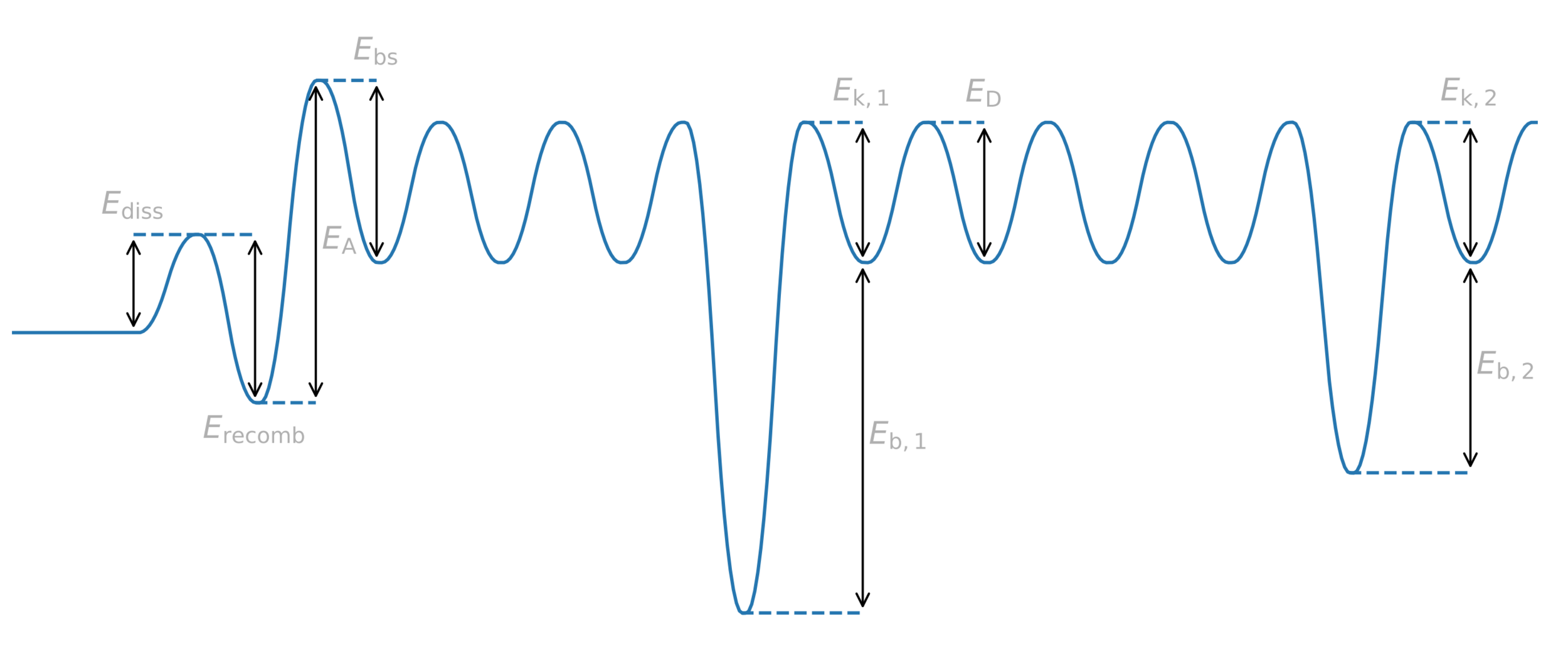
H
Trap = anything binding to H
- vacancy
- grain boundary
- impurity
- chemical reaction
- ...
Trapping
H
Potential energy
Distance
Diffusion barrier
Energy barrier = activation energy
Trap binding energy
Trapping energy
Common assumption:
\( E_k = E_D \)
Trapping
0D
Since \(n_\mathrm{trap} = n_\mathrm{free \ trap} + c_\mathrm{t} \)
Trapping
0D
Total concentration of traps
Trapping
0D
With diffusion
and
1 trap
Trapping
N traps
McNabb & Foster model
Trapping
Other models assume traps can hold more than one H
Many of these processes are thermally activated
Recombination
Dissociation
Absorption
Trapping
Detrapping
Diffusion
Arrhenius law
Pre-exponential factor
Activation energy (eV/H)
Temperature (K)
Boltzmann constant (eV/H/K)
Arrhenius law
Pre-exponential factor
Activation energy (J/mol)
Temperature (K)
Gas constant (J/mol/K)
Conversion:
Arrhenius law
\( 1/T \) (1/K)
Arrhenius law
Intercept
+ Slope
Y =
X
Arrhenius law
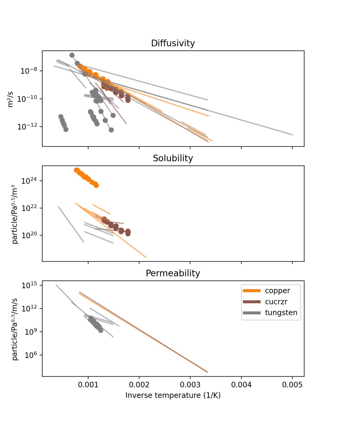
Arrhenius parameters:
- Diffusivity
- Solubility
- Permeability
- Recombination coeff.
- Dissociation coeff.
- Trapping rate
- Detrapping rate