Supervised Learning
ML in Feedback Sys #2
Prof Sarah Dean
Announcements
- Sign up to scribe
- Rank preferences for paper presentations
- Email me about first paper presentations 9/12 and 9/14
- HSNL18 Fairness Without Demographics in Repeated Loss Minimization
- PZMH20 Performative Prediction
- Required: meet with Atul at least 2 days before you are scheduled to present
- Working in pairs/groups, self-assessment

training data
\(\{(x_i, y_i)\}\)
model
\(f:\mathcal X\to\mathcal Y\)
policy
observation
action
ML in Feedback Systems

training data
\(\{(x_i, y_i)\}\)
model
\(f:\mathcal X\to\mathcal Y\)
observation
prediction
Supervised learning
\(\mathcal D\)
sampled i.i.d. from \(\mathcal D\)
\(x\sim\mathcal D_{x}\)
Goal: for new sample \(x,y\sim \mathcal D\), prediction \(\hat y = f(x)\) is close to true \(y\)
Predictions via Risk Mimization
Goal: for new sample \(x,y\sim \mathcal D\), prediction \(\hat y = f(x)\) is close to true \(y\)
\(\ell(y,\hat y)\) measures "loss" of predicting \(\hat y\) when it's actually \(y\)
Encode our goal in risk minimization framework:
$$\min_{f\in\mathcal F}\mathcal R(f) = \mathbb E_{x,y\sim\mathcal D}[\ell(y, f(x))]$$
$$\hat \theta = \arg\min \sum_{i=1}^N(-\theta^\top x_i\cdot y_i)_+$$
predict \(\hat f(x) = \mathbb 1\{\hat\theta^\top x \geq t\}\)

Ex: targeted job ads
No fairness through unawareness!
\(x_i=\) demographic info and browsing history
\(y_i=\) clicked (1) or not (-1)

The index of \(\hat\theta\) corresponding to "female" is negative!
The index of \(\hat\theta\) corresponding to "visited website for women's clothing store" is negative!
Statistical Classification Criteria

Accuracy
\(\mathbb P( \hat Y = Y)\) = ________
Positive rate
\(\mathbb P( \hat Y = 1)\) = ________
False positive rate
\(\mathbb P( \hat Y = 1\mid Y = 0)\) = ________
False negative rate
\(\mathbb P( \hat Y = 0\mid Y = 1)\) = ________
Positive predictive value
\(\mathbb P( Y = 1\mid\hat Y = 1)\) = ________
Negative predictive value
\(\mathbb P( Y = 0\mid\hat Y = 0)\) = ________
\(X\)
\(Y=1\)
\(Y=0\)
\(f(X)\)
\(3/4\)
\(9/20\)
\(1/5\)
\(3/10\)
\(7/9\)
\(8/11\)
Non-discrimination Criteria
- Informally: predictor should treat individuals the "same" across groups
- Formally: equalize positive rate, error rate, or predictive value across groups
Independence: prediction does not depend on \(a\)
\(\hat y \perp a\)
e.g. ad displayed at equal rates across gender
Separation: given outcome, prediction does not depend on \(a\)
\(\hat y \perp a~\mid~y\)
e.g. ad displayed to interested users at equal rates across gender
Sufficiency: given prediction, outcome does not depend on \(a\)
\( y \perp a~\mid~\hat y\)
e.g. users viewing ad are interested at equal rates across gender
In addition to features \(x\) and labels \(y\), individuals have protected attribute \(a\) (e.g. gender, race)
Ref: Ch 2 of Hardt & Recht, "Patterns, Predictions, and Actions" mlstory.org; Ch 3 of Barocas, Hardt, Narayanan "Fairness and Machine Learning" fairmlbook.org.
Ex: Pre-trial Detention

- COMPAS: a criminal risk assessment tool used in pretrial release decisions
- \(x\) survey about defendant
- \(\hat y\) designation as high- or low-risk
- Audit of data from Broward county, FL
- \(a\) race of defendant
- \(y\) recidivism within two years
“Black defendants who did not recidivate over a two-year period were nearly twice as likely to be misclassified. [...] White defendants who re-offended within the next two years were mistakenly labeled low risk almost twice as often.”
Ex: Pre-trial Detention

“In comparison with whites, a slightly lower percentage of blacks were ‘Labeled Higher Risk, But Didn’t Re-Offend.’ [...] A slightly higher percentage of blacks were ‘Labeled Lower Risk, Yet Did Re-Offend.”’

\(\mathbb P(\hat y = 1\mid y=0, a=\text{Black})> \mathbb P(\hat y = 1\mid y=0, a=\text{White}) \)
\(\mathbb P(\hat y = 0\mid y=1, a=\text{Black})< \mathbb P(\hat y = 0\mid y=1, a=\text{White}) \)
\(\mathbb P(y = 0\mid \hat y=1, a=\text{Black})\approx \mathbb P( y = 0\mid \hat y=1, a=\text{White}) \)
\(\mathbb P(y = 1\mid \hat y=0, a=\text{Black})\approx \mathbb P( y = 1\mid \hat y=0, a=\text{White}) \)
COMPAS risk predictions do not satisfy separation
Ex: Pre-trial Detention

COMPAS risk predictions do satisfy sufficiency

Achieving Nondiscrimination Criteria
- Pre-processing: remove correlations between \(a\) and features \(x\) in dataset.
-
Pre-processing: remove correlations between \(a\) and features \(x\) in dataset.
- Requires knowledge of \(a\) during data cleaning
Achieving Nondiscrimination Criteria
- Pre-processing: remove correlations between \(a\) and features \(x\) in dataset.
-
In-processing: modify learning algorithm to respect criteria.
- Requires knowledge of \(a\) at training time
Achieving Nondiscrimination Criteria
- Pre-processing: remove correlations between \(a\) and features \(x\) in dataset.
- In-processing: modify learning algorithm to respect criteria.
- Post-processing: adjust thresholds in group-dependent manner.
Achieving Nondiscrimination Criteria
- Pre-processing: remove correlations between \(a\) and features \(x\) in dataset.
- In-processing: modify learning algorithm to respect criteria.
-
Post-processing: adjust thresholds in group-dependent manner.
- Requires knowledge of \(a\) at decision time
Achieving Nondiscrimination Criteria
Limitations of Nondiscrimination Criteria
- Tradeoffs: It is impossible to simultaneously satisfy separation and sufficiency if populations have different base rates


Kleinberg & Raghavan, Inherent Trade-Offs in the Fair Determination of Risk Scores
Limitations of Nondiscrimination Criteria
- Tradeoffs: It is impossible to simultaneously satisfy separation and sufficiency if populations have different base rates
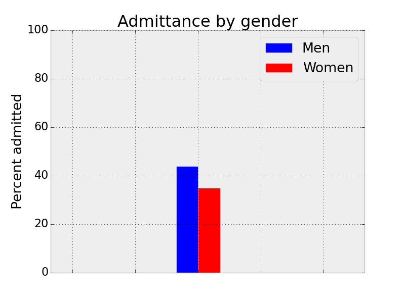
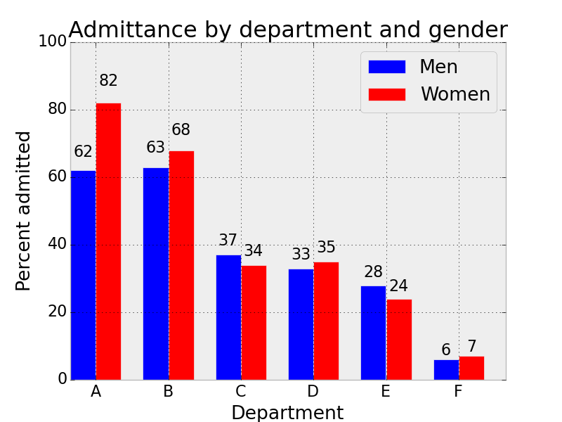
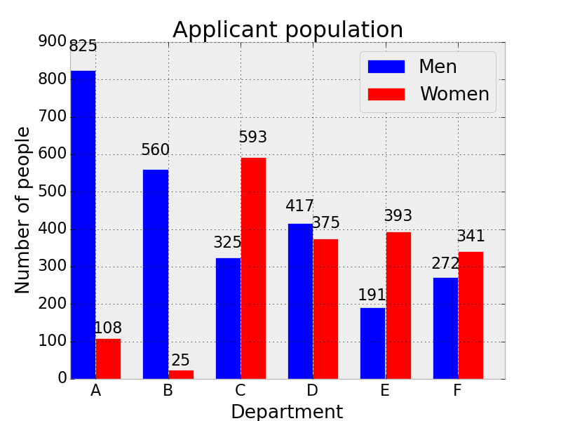
- Observational: Statistical criteria can measure only correlation; intuitive notions of discrimination involve causation, which requires careful modelling


Simpson's Paradox, Cory Simon
Limitations of Nondiscrimination Criteria
- Tradeoffs: It is impossible to simultaneously satisfy separation and sufficiency if populations have different base rates
- Observational: Statistical criteria can measure only correlation; intuitive notions of discrimination involve causation, which requires careful modelling
- Unclear legal grounding: While algorithmic decisions may have disparate impact, achieving criteria involves disparate treatment
Barocas & Selbst, Big Data's Disparate Impact
Limitations of Nondiscrimination Criteria
- Tradeoffs: It is impossible to simultaneously satisfy separation and sufficiency if populations have different base rates
- Observational: Statistical criteria can measure only correlation; intuitive notions of discrimination involve causation, which requires careful modelling
- Unclear legal grounding: While algorithmic decisions may have disparate impact, achieving criteria involves disparate treatment
- Limited view: focusing on risk prediction might miss the bigger picture of how these tools are used by larger systems to make decisisons
Discrimination Beyond Classification


image cropping
facial recognition
information retrieval
generative models
Empirical Risk Minimization
- define loss
- do ERM
performance depends on risk \(\mathcal R(f)\)
$$\hat f = \min_{f\in\mathcal F} \frac{1}{n} \sum_{i=1}^n \ell(y_i, f(x_i))$$
\(\{\)
\(\mathcal R_N(f)\)
(with fairness constraints)

training data
\(\{(x_i, y_i)\}\)
model
\(f:\mathcal X\to\mathcal Y\)
\(\mathcal D\)
Sample vs. population
Fundamental Theorem of Supervised Learning:
- The risk is bounded by the empirical risk plus the generalization error. $$ \mathcal R(f) \leq \mathcal R_N(f) + |\mathcal R(f) - \mathcal R_N(f)|$$
Empirical risk minimization
$$\hat f = \min_{f\in\mathcal F} \frac{1}{n} \sum_{i=1}^n \ell(y_i, f(x_i))$$
\(\{\)
\(\mathcal R_N(f)\)
1. Representation
2. Optimization
3. Generalization
Case study: linear regression
At first glance, linear representation seems limiting
Least-squares linear regression models \(y\approx \theta^\top x\)
$$\min_{\theta\in\mathbb R^d} \frac{1}{n}\sum_{i=1}^n \left(\theta^\top x_i - y_i\right)^2$$
but we can encode rich representations by expanding the features (increasing \(d\))
\(y = (x-1)^2\)
\(y = \begin{bmatrix}1\\-2\\1\end{bmatrix}^\top \begin{bmatrix}1\\x\\x^2\end{bmatrix} \)
\(\varphi(x)\)
\(\{\)
For more, see Ch 4 of Hardt & Recht, "Patterns, Predictions, and Actions" mlstory.org.
Case study: linear regression
one global min
infinitely many global min
local and global min
Optimization is straightforward due to differentiable and convex risk
$$\min_{\theta\in\mathbb R^d} \frac{1}{n}\sum_{i=1}^n \left(\theta^\top x_i - y_i\right)^2$$
strongly convex
convex
nonconvex
Case study: linear regression
Derivation of optimal solution
$$\hat\theta\in\arg\min_{\theta\in\mathbb R^d} \frac{1}{n}\sum_{i=1}^n \left(\theta^\top x_i - y_i\right)^2$$
first order optimality condition: \( \displaystyle \sum_{i=1}^n x_i x_i^\top\hat \theta = \sum_{i=1}^n y_ix_i \)
min-norm solution: \( \displaystyle \hat\theta = \left( \sum_{i=1}^n x_i x_i^\top\right)^\dagger\sum_{i=1}^n y_ix_i \)
Case study: linear regression
Proof: exercise. Hint: consider the span of the \(x_i\).
Iterative optimization with gradient descent $$\theta_{t+1} = \theta_t - \alpha\sum_{i=1}^n (\theta_t^\top x_i - y_i)x_i$$
Claim: suppose \(\theta_0=0\) and GD converges to a minimizer. Then it converges to the minimum norm solution.
Case study: linear regression
Generalization: under the fixed design generative model, \(\{x_i\}_{i=1}^n\) are fixed and
\(y_i = \theta_\star^\top x_i + v_i\) with \(v_i\) i.i.d. with mean \(0\) and variance \(\sigma^2\)
\(\mathcal R(\theta) = \frac{1}{n}\sum_{i=1}^n \mathbb E_{y_i}\left[(x_i^\top \theta - y_i)^2\right]\)
Claim: when features span \(\mathbb R^d\), the excess risk \(\mathcal R(\hat\theta) -\mathcal R(\theta_\star) =\frac{\sigma^2 d}{n}\)
- First, \(\mathcal R(\theta) = \frac{1}{n}\|X(\theta-\theta_\star)\|_2^2 + \sigma^2\)
- Then, \(\|X(\hat\theta-\theta_\star)\|_2^2 = v^\top X(X^\top X)^{-1}X^\top v\)
- Then take expectation.
Case study: linear regression
Exercises:
- For the same generative model and a new fixed \(x_{n+1}\), what is the expected loss \(\mathbb E_y[(\hat \theta^\top x_{n+1} - y_{n+1})^2]\)? Can you interpret the quantities?
- In the random design setting, we take each \(x_i\) to be drawn i.i.d. from \(\mathcal N(0,\Sigma)\) and assume that \(v_i\) is also Gaussian. The risk is then $$\mathcal R(\theta) = \mathbb E_{x, y}\left[(x^\top \theta - y)^2\right].$$ What is the excess risk of \(\hat\theta\) in terms of \(X^\top X\) and \(\Sigma\)? What is the excess risk in terms of \(\sigma^2, n, d\) (ref 1, 2)?
Recap
- Non-discrimination criteria
- independence, separation, and sufficiency
- Least-squares regression
- representation, optimization, generalization
Next time: online learning with linear least-squares case study