Nonlinear Dynamics and Linearization
ML in Feedback Sys #5
Fall 2025, Prof Sarah Dean
What about some nonlinear approx?
I.e. train deep network so $$\hat x_{t+1} = NN(\hat x_t)$$
Can we predict stability of predictions?
unstable
stable
Nonlinear dynamics stability
"What we do"
- Given: the nonlinear difference equation \(s_{t+1} = F(s_t)\) and a fixed point \(s_{eq}\)
- Compute the Jacobian $$ J(s) = \begin{bmatrix}\frac{\partial F_1}{\partial s_1} & \dots & \frac{\partial F_1}{\partial s_d} \\ \vdots & \ddots & \vdots \\ \frac{\partial F_d}{\partial s_1} &\dots & \frac{\partial F_d}{\partial s_d}\end{bmatrix}$$
- Compute the linearized dynamics by evaluating \(J(s_{eq})\)
- Assess stability: with \(\max_{i=1,..,d} |\lambda_i(J(s_{eq}))|\)
- \(> 1 \implies\) unstable
- \(< 1 \implies\) stable
- \(=1 \implies\) inconclusive
\(\mathbb C\)
stable
unstable
inconclusive
\(1\)
Consider the dynamics of gradient descent on a twice differentiable function \(\ell:\mathbb R^d\to\mathbb R^d\)
\(\theta_{t+1} = \theta_t - \alpha\nabla \ell(\theta_t)\)
Example: gradient descent
- Equilibria occur when \(\nabla \ell(\theta_{eq}) = 0\), i.e. at critical points
-
Review: critical point classification in terms of second derivatives
- positive definite: (local) min
- negative definite: (local) max
- both positive and negative: saddle point
- zero: indeterminate or degenerate
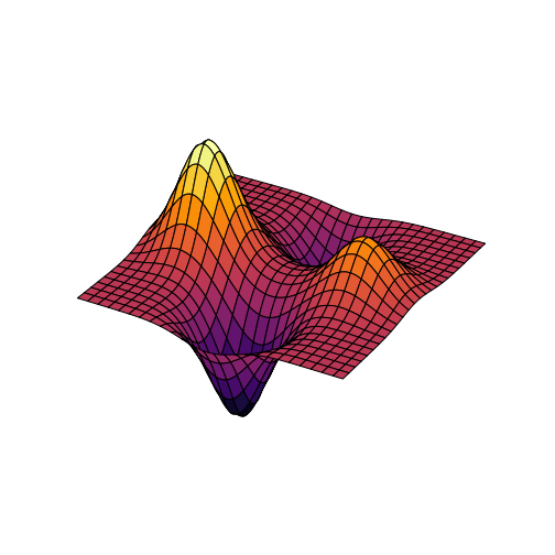
global max
local max
global min
local min
saddle
Consider the dynamics of gradient descent on a twice differentiable function \(\ell:\mathbb R^d\to\mathbb R^d\)
\(\theta_{t+1} = \theta_t - \alpha\nabla \ell(\theta_t)\)
Example: gradient descent
- Equilibria occur when \(\nabla \ell(\theta_{eq}) = 0\), i.e. at critical points
- Jacobian \(J(\theta) = I - \alpha \nabla^2 \ell(\theta)\)
- Let \(\{\gamma_i\}_{i=1}^d\) be the eigenvalues of the Hessian \(\nabla^2 \ell(\theta_{eq})\)
- Then the eigenvalues of the Jacobian are \(1-\alpha\gamma_i\)
-
if any \(\gamma_i\leq 0\), \(\theta_{eq}\) is not strictly stable
-
i.e. saddle, local maximum, or degenerate critical point of \(\ell\)
-
- as long as \(\alpha<\frac{1}{\gamma_i}\) for all \(i\), \(\theta_{eq}\) is stable
-
global max
local max
global min
local min
saddle
Consider the dynamics of gradient descent on a twice differentiable function \(\ell:\mathbb R^d\to\mathbb R^d\)
\(\theta_{t+1} = \theta_t - \alpha\nabla \ell(\theta_t)\)
Example: gradient descent
- Equilibria occur when \(\nabla \ell(\theta_{eq}) = 0\), i.e. at critical points
- Only (non-degenerate) local minima are stable
global max
local max
global min
local min
saddle
Outline
"Why we do it"
- Linear approximations
- Lyapunov stability theory
- Limit cycles and chaos
1D Example
Consider linear approximation of nonlinear dynamics
states tend to evolve away from middle equilibrium and towards right (or left)
middle equilibrium has a slope \(>1\) while right/left have slopes \(<1\)
Linearization example
example: discrete-time damped pendulum
\(\theta_{t+1} = \theta_t + h \omega_t\)
\(\omega_{t+1} =\omega_t + h\left(\frac{g}{\ell}\sin\theta_t-d\omega_t\right)\)
angle \(\theta\)
angular velocity \(\omega\)
gravity
length \(\ell\)
\(\approx (1-dh)\omega_t + h\frac{g}{\ell}(\sin \theta_{eq}+\cos\theta_{eq}(\theta-\theta_{eq})\)
\(\sin x\approx \sin x_0 + \cos x_0(x - x_0)\)

equilibria at \(\theta=k\pi\) for \(k\in\mathbb N\)
Consider linear approximation of nonlinear dynamics
Linearization example
example: discrete-time damped pendulum
angle \(\theta\)
angular velocity \(\omega\)
gravity
length \(\ell\)
$$\begin{bmatrix}\theta_{t+1}-\theta_{eq}\\ \omega_{t+1}\end{bmatrix} \approx \begin{bmatrix} 1 & h\\ h \frac{g}{\ell}\cos(\theta_{eq})& 1-dh\end{bmatrix}\begin{bmatrix}\theta_{t}-\theta_{eq}\\ \omega_{t}\end{bmatrix} $$
at \(\theta_{eq}=0\), real eigenvalues \(0<\lambda_2<1<\lambda_1\)
at \(\theta_{eq}=\pi\), complex eigenvalues with \(|\lambda|<1\) for small \(d\)
Exercise: work out the details of this analysis (simulation notebook)
Consider linear approximation of nonlinear dynamics
\(\lambda = 1-h\frac{d}{2} \pm h\sqrt{(\frac{d}{2})^2+\frac{g}{\ell}\cos(\theta_{eq})}\)
Linearization example
example: discrete-time damped pendulum
angle \(\theta\)
angular velocity \(\omega\)
gravity
length \(\ell\)
at \(\theta_{eq}=0\), real eigenvalues \(0<\lambda_2<1<\lambda_1\)
at \(\theta_{eq}=\pi\), complex eigenvalues with \(|\lambda|<1\) for small \(d\)
Consider linear approximation of nonlinear dynamics
Linearization via Taylor Series:
\(s_{t+1} = F(s_t) \)
- \(=F(s_{eq}) + J(s_{eq}) (s_t - s_{eq}) \) + higher order terms
- \(=s_{eq} + J(s_{eq}) (s_t - s_{eq}) \) + higher order terms
- \(\implies s_{t+1}-s_{eq} \approx J(s_{eq})(s_t-s_{eq})\)
Vector-valued linearization
The Jacobian \(J\) of \(G:\mathbb R^{n}\to\mathbb R^{m}\) is defined as $$ J(x) = \begin{bmatrix}\frac{\partial G_1}{\partial x_1} & \dots & \frac{\partial G_1}{\partial x_n} \\ \vdots & \ddots & \vdots \\ \frac{\partial G_m}{\partial x_1} &\dots & \frac{\partial G_m}{\partial x_n}\end{bmatrix}$$
Outline
"Why we do it"
- Linear approximations
- Lyapunov stability theory
- Limit cycles and chaos
Definition: A Lyapunov function \(V:\mathcal S\to \mathbb R\) for \(F\) is continuous and
- (positive definite) \(V(0)=0\) and \(V(0)>0\) for all \(s\in\mathcal S - \{0\}\)
- (decreasing) \(V(F(s)) - V(s) \leq 0\) for all \(s\in\mathcal S\)
- Optionally,
- (strict) \(V(F(s)) - V(s) < 0\) for all \(s\in\mathcal S-\{0\}\)
- (global) \(\|s\|_2\to \infty \implies V(s)\to\infty\)
Lyapunov functions

Reference: Bof, Carli, Schenato, "Lyapunov Theory for Discrete Time Systems"
Lyapunov Stability Theory
Theorem (1.2, 1.4): Suppose that \(F\) is locally Lipschitz, \(s_{eq}=0\) is a fixed point, and \(V\) is a Lyapunov function. Then, \(s_{eq}=0\) is
- stable
- asymptotically stable if \(V\) satisfies the strict property
- globally asymptotically stable if \(V\) satisfies the strict and global properties
Reference: Bof, Carli, Schenato, "Lyapunov Theory for Discrete Time Systems"
Quadratic Lyapunov functions
- Stable matrices have quadratic Lyapunov functions of the form \(V(s) = s^\top P s\) (Theorem 3.2)
- For example, \(P = \sum_{t=0}^\infty (F^\top)^t F^t\)
-
Exercise: show that the above is a strict and global Lyapunov function for \(s_{t+1}= F s_t\).
- positive definite: argue why \(P\succ 0\)
- decreasing: argue why \(V(Fs) - V(s) \leq 0\) for all \(s\)
Linearization Stability Test
Theorem (3.3): Suppose \(F\) is locally Lipschitz, \(0\) is a fixed point, and let \(\{\lambda_i\}_{i=1}^d\subset \mathbb C\) be the eigenvalues of the Jacobian \(J(0)\). Then \(0\) is
- asymptotically stable if \(\max_{i\in[d]}|\lambda_i|<1\)
- unstable if \(\max_{i\in[d]}|\lambda_i|> 1\)
Proof sketch.
- When Jacobian \(J(0)\) is stable, can define \(P = \sum_{t=0}^\infty (J(0)^\top)^t J(0)^t\). Then use \(s^\top P s\) to construct a strict Lyapunov function for \(s_{t+1} = F(s_t)\).
\(\mathbb C\)
stable
unstable
inconclusive
\(1\)
Outline
"Why we do it"
- Linear approximations
- Lyapunov stability theory
- Limit cycles and chaos
- Nonlinear dynamics can display complex behaviors beyond stable/unstable equilibria
- Example: logistic map (simulation notebook) $$s_{t+1}= rs_t(1-s_t)$$
Complex dynamic behaviors
- \(r=0.5\) stable at \(s=0\)
-
\(r=1.5\) stable at \(s=\frac{1}{3}\)
-
\(r=3.25\) limit cycle
-
\(r=3.75\) chaotic
Next time: learning nonlinear models
Recap
References: Bof, Carli, Schenato, "Lyapunov Theory for Discrete Time Systems"
- Nonlinear stability via linearization
- Theoretical tool: Lyapunov functions
Announcements
- Second assignment due Thursday
- My office hours:
- informally after lecture walking to Gates
- by appointment after lecture in my office 424 Gates