Hidden Markov Models
ML in Feedback Sys #9
Fall 2025, Prof Sarah Dean
Discrete Filtering
"What we do"
- Given transition probabilities, observation probabilities, and initial state distribution \(\mu_0\), $$P_{ij} = \mathbb P\{S_{t+1}=j|S_t=i\} ,\qquad B_{ij}=\mathbb P\{Y_{t}=j|S_t=i\}$$
- For streaming observations \(y_t\), \(t\geq 0\):
- Predict state distribution: \( \mu_{t+1|t} = P^\top \mu_{t|t}\)
- Update state distribution: $$ \mu_{t+1|t+1}= Be_{y_{t+1}} \odot \mu_{t+1|t} / (e_{y_{t+1}}^\top B^\top \mu_{t+1|t})$$
- Predict distribution of future observations $$ y_{t+k|t}\sim B^\top (P^\top)^k\mu_{t|t}$$
Discrete Filtering
"Why we do it"
-
Consider a hidden Markov model with transitions \(P\) and observation probabilities \(B\) $$ S_{t+1} \sim P^\top e_{s_t},\quad Y_t \sim B^\top e_{s_t} $$
-
Fact: the filtering algorithm computes the posterior $$ \mathbb P\{S_{t}=i|y_0,...,y_t\}=\mu_{t|t}[i] $$
-
Fact: the relationship between the observations and the estimated state is bilinear, so predictions depend polynomially on past observations
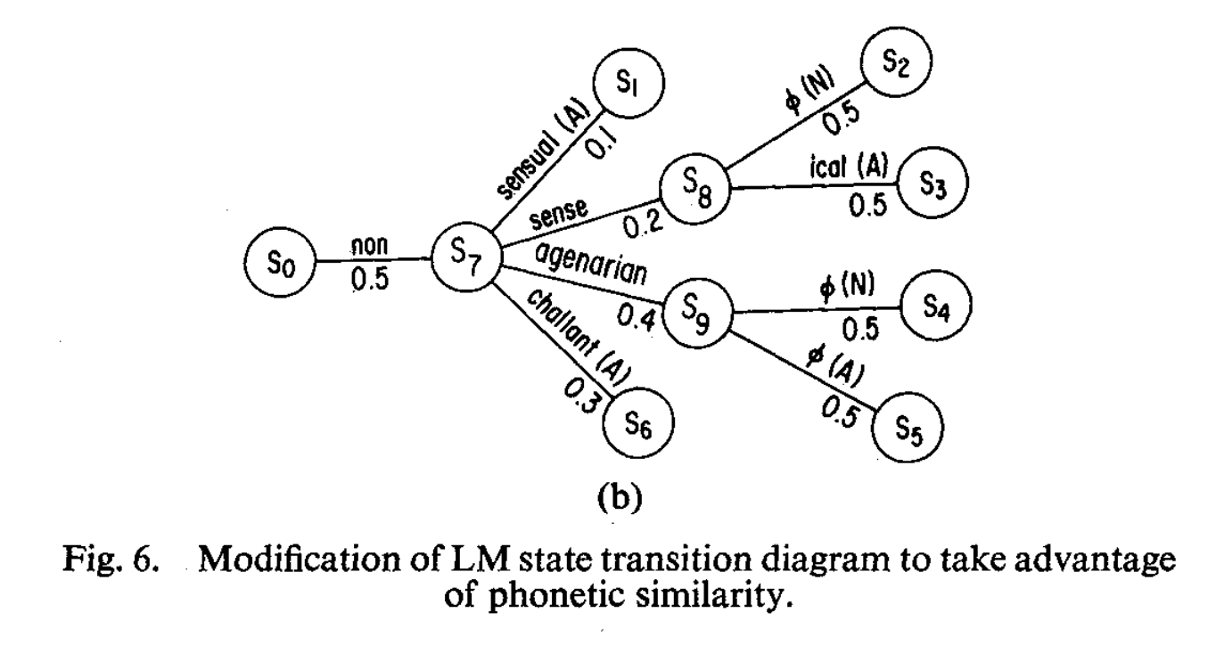
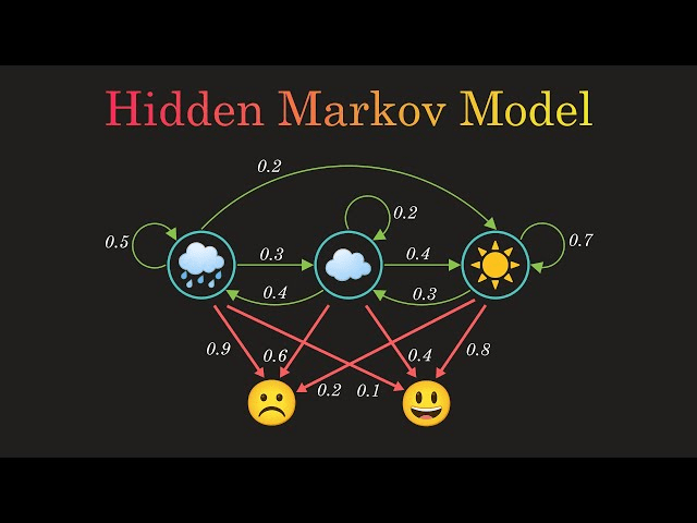
Hidden Markov models
- Model in which a Markovian state is latent
- Discrete setting with \(|\mathcal S|\) states and \(|\mathcal Y|\) observations
- Specified by \(|\mathcal S|^2+|\mathcal S||\mathcal Y|\) transition and observation probabilities $$P_{ij} = \mathbb P\{S_{t+1}=j|S_t=i\} ,\qquad B_{ij}=\mathbb P\{Y_{t}=j|S_t=i\}$$
- For discrete states and observations, given that \(S_t=s_t\), $$ S_{t+1} \sim P^\top e_{s_t},\quad Y_t \sim B^\top e_{s_t} $$
Hidden Markov models
- Model in which a Markovian state is latent
- Discrete setting with \(|\mathcal S|\) states and \(|\mathcal Y|\) observations
- Specified by \(|\mathcal S|^3|\mathcal Y|\) transition and observation probabilities $$P_{ij} = \mathbb P\{S_{t+1}=j|S_t=i\} ,\qquad B_{ij}=\mathbb P\{Y_{t}=j|S_t=i\}$$
- For discrete states and observations, given that \(S_t\sim \mu_t\), $$ S_{t+1} \sim P^\top \mu_t,\quad Y_t \sim B^\top \mu_t$$
- Recall the stationary distribution and convergence are determined by eigenvectors/values of \(P\)
- Fact: the filtering algorithm computes the posterior $$ \mathbb P\{S_{t}=i|y_0,...,y_t\}=\mu_{t|t}[i] $$
- For streaming observations \(y_t\), \(t\geq 0\):
- Prediction step: \( \mu_{t+1|t} = P^\top \mu_{t|t}\)
- \(\mathbb P\{S_{t+1}=i|y_{0:t}\} = \sum_{j=1}^{|\mathcal S|} \mathbb P\{S_{t+1}=i|S_{t}=j\} \mathbb P\{S_{t}=j|y_{0:t}\}\)
- Update step: \( \mu_{t+1|t+1}= Be_{y_{t+1}} \odot \mu_{t+1|t} / (e_{y_{t+1}}^\top B^\top \mu_{t+1|t})\)
- \(\mathbb P\{S_{t+1}=i|y_{0:t+1}\} \propto \mathbb P\{Y_{t+1}=y_{t+1}|S_{t+1}=i\} \mathbb P\{S_{t+1}=i|y_{0:t}\} \)
- Prediction step: \( \mu_{t+1|t} = P^\top \mu_{t|t}\)
Posterior distribution
Linear recursion in state
- Computations are linear function of the state distribution
- Predict is \(O(|\mathcal S|^2)\): \( \mu_{t+1|t} = P^\top \mu_{t|t}\)
- Update is \(O(|\mathcal S|^2)\) $$ \mu_{t+1|t+1}= Be_{y_{t+1}} \odot \mu_{t+1|t} / (e_{y_{t+1}}^\top B^\top \mu_{t+1|t})$$
- Comparing with Kalman filter:
- Predict is \(O(d_s^3)\)
\(\hat s_{t\mid t-1} =F\hat s_{t-1\mid t-1},~~P_{t\mid t-1} = FP_{t-1\mid t-1} F^\top + \Sigma_w\) - Update is \(O(d_s^2 d_y + d_y^3)\)
\(L_{t} = P_{t\mid t-1}H^\top ( HP_{t\mid t-1} H^\top+\Sigma_v)^{-1}\)
\(\hat s_{t\mid t} = \hat s_{t\mid t-1}+ L_{t}(y_{t}-H\hat s_{t\mid t-1}),~~ P_{t\mid t} = (I - L_{t}H)P_{t\mid t-1}\)
- Predict is \(O(d_s^3)\)
Linear recursion in state
- Computations are linear function of the state distribution
- Predict: \( \mu_{t+1|t} = P^\top \mu_{t|t}\) is \(O(|\mathcal S|^2)\)
- Update is \(O(|\mathcal S|^2)\) $$ \mu_{t+1|t+1}= Be_{y_{t+1}} \odot \mu_{t+1|t} / (e_{y_{t+1}}^\top B^\top \mu_{t+1|t})$$
- Let \(D_{y_t} = \mathrm{diag}(Be_{y_{t}})P^\top\), then $$\mu_{t+1|t+1}= D_{y_{t+1}} \mu_{t|t} / (\mathbb 1^\top D_{y_{t+1}} \mu_{t|t})$$
- Unrolled recursion: $$\mu_{t|t}= D_{y_t}D_{y_{t-1}}...D_{y_0} \mu_{0} / (\mathbb 1^\top D_{y_t}D_{y_{t-1}}...D_{y_0} \mu_{0}) $$
- Predictions \( y_{t+k|t}\sim B^\top (P^\top)^k\mu_{t|t}\)
- Update is bilinear in state and observation $$\mu_{t+1|t+1}= D_{y_{t+1}} \mu_{t|t} / (\mathbb 1^\top D_{y_{t+1}} \mu_{t|t})$$
- Predictions are given by $$ y_{t+k|t}\sim B^\top (P^\top)^kD_{y_t}D_{y_{t-1}}...D_{y_0} \mu_{0} / (\mathbb 1^\top D_{y_t}D_{y_{t-1}}...D_{y_0} \mu_{0}) $$
- where we have \(D_{y_t} = \mathrm{diag}(Be_{y_{t}})P^\top\)
- Dependence on product of observations
- Compare with KF recursion, where update was linear $$\hat y_{t|t-1} = H\Big(\prod_{k=0}^{t-1} F_{L,k}\Big) \hat s_{0}+ \sum_{k=1}^{t}H \Big(\prod_{\ell=0}^{k-1} F_{L,\ell}\Big) L_{t-1}y_{t-k+1}$$
- where \(F-L_tHF\) is independent of observations (since observation noise is independent)
- Linear dependence on observations
Bilinear dependence on observation
- Update is bilinear in state and observation $$\mu_{t+1|t+1}= D_{y_{t+1}} \mu_{t|t} / (\mathbb 1^\top D_{y_{t+1}} \mu_{t|t})$$
- Predictions are given by $$ y_{t+k|t}\sim B^\top (P^\top)^kD_{y_t}D_{y_{t-1}}...D_{y_0} \mu_{0} / (\mathbb 1^\top D_{y_t}D_{y_{t-1}}...D_{y_0} \mu_{0}) $$
- where we have \(D_{y_t} = \mathrm{diag}(Be_{y_{t}})P^\top\)
- Dependence on product of observations
- Still have that \(\epsilon\) approximation is possible with a finite \(L\) window (Sharan et al., 2016)
- However would need to use polynomial features to represent as some linear \(y_{t+k|t}\sim\Theta^\top\varphi(y_0,...,y_{L-1})\)
- scaling exponentially in \(L\) and \(|\mathcal Y|\)
Bilinear dependence on observation
- We focus on filtering and output prediction
- This is known as "forward" algorithm for HMM inference
- Other important tasks include:
- Smoothing ("backwards" algorithm) computes for \(k\leq t\) $$\mathbb P\{S_k|y_0,...,y_t\}$$
- Maximum a posteriori state sequence with "Viterbi algorithm" is an example of dynamic programming $$\max_{s_0,...,s_t} \mathbb P\{S_k=s_k|y_{0:t}\}$$
- For PO-LDS, these tasks amount to solving the full least-squares problem to compute \(\hat s_{k|t}\)
Other HMM tasks
- Linear least squares for predicting (vector valued) labels \(y\) from features \(x\)
- Categorical/discrete data with one-hot embeddings
- Works for nonlinear phenomena, just need a nonlinear feature transformation/kernel
- When data comes in the form of a sequence, how do we determine labels and features?
- Use elements of sequence as labels \(y_t\)
- Use previous \(L\) as features \(y_{t-1:t-L}\)
- We justify validity so far with theory on
- Optimization: convexity and regularization
- Representation: for dynamical systems, Markov chains, and partial observations
What we have covered so far
- Linear least squares for predicting (vector valued) labels \(y\) from features \(x\)
- For sequence data: use autoregressive models
- We justify validity so far with theory on
- Optimization: convexity and regularization
- Representation: for dynamical systems, Markov chains, and partial observations
- To further judge validity, we need to think about generalization
- There is no substitute for real world evaluation!
- We will consider generalization theory next lecture
What we have covered so far
Reference: Chapter 17 of Machine Learning: A Probabilistic Perspective
Recap
- Hidden Markov models
- Linear/bilinear prediction
Next time: generalization and online learning
Announcements
- Fourth assignment due Thursday
- Next week: discuss projects & paper presentations (see Syllabus)