Model Predictive Linear Quadratic Control
ML in Feedback Sys #12
Fall 2025, Prof Sarah Dean

policy
\(\pi_t:\mathcal S\to\mathcal A\)
observation
\(s_t\)
accumulate
\(\{(s_t, a_t, c_t)\}\)
Action in a dynamic world
Goal: select actions \(a_t\) to bring environment to low-cost states
action
\(a_{t}\)
\(F\)
\(s\)
Model Predictive Control
"What we do"
- Given a model \(F:\mathcal S\times \mathcal A\to\mathcal S\), cost \(c:\mathcal S\times \mathcal A\to\mathbb R\), planning horizon \(H\)
- For \(t=1,2,...\)
- Observe the state \(s_t\)
- Solve the optimization problem
- Take action \(a_t=a^\star_0(s_t)\)
\( \underset{a_0,\dots,a_H }{\min}\) \(\displaystyle\sum_{k=0}^H c(s_k, a_k)\)
\(\text{s.t.}~~s_0=s_t,~~s_{k+1} = F(s_k, a_k)\)
\([a_0^\star,\dots, a_{H}^\star](s_t) = \arg\)
model predicts the (action-dependent) trajectory
Model Predictive Control
"Why we do it"
- Fact 1: MPC is a flexible control strategy that is useful in many contexts.
- Fact 2: When costs are quadratic and dynamics are linear, MPC selects an action which depends linearly on the state. $$a_t^{MPC}=K_{MPC}s_t$$
- Fact 3: In the LQ setting, the optimal policy \(\pi^\star_t:\mathcal S\to\mathcal A\) for the stochastic optimal control problem is linear in the state. $$\pi^\star_t(s) = K^\star_t s$$
- Fact 4: The action selected by MPC is equal to that of the optimal policy for certain planning horizons or terminal costs. $$K_{MPC}\approx K^\star_t$$
- Flexible: any* model, any* objective (including constraints)
- easily incorporate time-varying dynamics, constraints (e.g. obstacles), costs (e.g. new incentives)
- *up to computational considerations
- Useful: good* performance (and safety) by definition
- *over the planning horizon
- Importance of replanning
- if state \(s_{t+1}\) does not evolve as expected (e.g. due to disturbances)
- plan over a shorter horizon than we operate \(H<T\)
Benefits of MPC
- Observe state
- Optimize plan
- For \(t=0,1,...\)
- Apply planned action
- For \(t=0,1,\dots\)
- Observe state
- Optimize plan
- Apply first planned action
Figure from slides by Borelli, Jones, Morari
Plan:
- minimize lap time
- subject to
- car dynamics
- staying within lane
- bounded acceleration
Example: racing
- For \(t=0,1,\dots\)
- Observe state
- Optimize plan
- Apply first planned action
Figure from slides by Borelli, Jones, Morari
Plan:
- minimize lap time
- subject to
- car dynamics
- staying within lane
- bounded acceleration
Example: racing
- For \(t=0,1,\dots\)
- Observe state
- Optimize plan
- Apply first planned action
Convexity of MPC
$$ \min_{a_{0:T}} ~~\sum_{k=0}^{T} c(s_k,a_k) \quad \text{s.t}\quad s_{k+1} = F s_k+ Ga_k $$
- Convex cost, linear constraints \(\implies\) Convex Program
s_vec = cvx.Variable((T*n, 1), name="s")
a_vec = cvx.Variable((T*p, 1), name="a")

# Linear dynamics constraint
constr = [s_vec[:n, :] == s_0]
for k in range(T):
    constr.append(s_vec[n*(k+1):n*(k+1+1)] == F*s_vec[n*k:n*(k+1),:] + G*a_vec[p*k:p*(k+1),:])

# Convex cost
objective = cost(s_vec, a_vec)

prob = cvx.Problem(cvx.Minimize(objective), constr)
prob.solve()
actions = np.array(a_vec.value)
map of how actions affect states
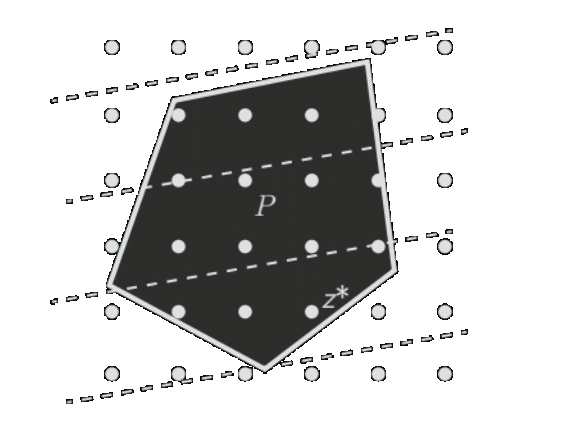
- Linear Program (LP): Linear costs and constraints, feasible set is polyhedron. $$\min_z c^\top z~~ \text{s.t.} ~~Gz\leq h,~~Az=b$$
-
Quadratic Program (QP): Quadratic cost and linear constraints, feasible set is polyhedron. Convex if \(P\succeq 0\). $$\min_z z^\top P z+q^\top z~~ \text{s.t.} ~~Gz\leq h,~~Az=b$$
- Nonconvex if \(P\nsucceq 0\).
- Mixed Integer Linear Program (MILP): LP with discrete constraints. $$\min_z c^\top z~~ \text{s.t.} ~~Gz\leq h,~~Az=b,~~z\in\{0,1\}^n$$
Types of optimization problems
Figures from slides by Goulart, Borelli


Convexity of MPC
$$ \min_{a_{0:T}} ~~\sum_{k=0}^{T} s_k^\top Qs_k + a_k^\top Ra_k \quad \text{s.t}\quad s_{k+1} = F s_k+ Ga_k $$
- Convex cost, linear constraints \(\implies\) Convex Program
- Quadratic cost, linear constraints \(\implies\) Quadratic Program
- Only equality constraints \(\implies\) substitute and solve with first order optimality condition
Fact 2: When costs are quadratic and dynamics are linear, MPC selects an action which depends linearly on the state. $$a_t^{MPC}=K_{MPC}s_t$$
- Note that state is linear in inputs and initial state $$\displaystyle s_{t} = F^t s_0+ \sum_{k=1}^{t}F^{k-1}Ga_{t-k}$$
- Equivalent minimization for some matrices \(M_1,M_2,M_3\) $$ \min_{\mathbf a} ~~ s_0^\top M_1 s_0 + s_0^\top M_2\mathbf a+ \mathbf a^\top M_3\mathbf a$$
- Quadratic minimization:
- \(\min_{\mathbf a} {\mathbf a}^\top M {\mathbf a} + m^\top {\mathbf a} + c\) for \(M\succ 0\)
- \(2M{\mathbf a}_\star + m = 0 \implies {\mathbf a}_\star = -\frac{1}{2}M^{-1} m\)
Closed form LQ MPC
The MPC Policy
\(F\)
\(s\)
\(s_t\)
\(a_t = a_0^\star(s_t)\)
\( \underset{a_0,\dots,a_H }{\min}\) \(\displaystyle\sum_{k=0}^H c(s_k, a_k)\)
\(\text{s.t.}~~s_0=s_t,~~s_{k+1} = F(s_k, a_k)\)
Fact 2: When costs are quadratic and dynamics are linear, MPC selects an action which depends linearly on the state. $$a_t^{MPC}=K_{MPC}s_t$$
Example
- Setting: UAV hover over to origin \(s_\star = (0,0)\)
- action: thrust right/left, state is pos/vel
- \(F(s_t, a_t) = \begin{bmatrix}1 & 1 \\ 0 & 1\end{bmatrix}s_t + \begin{bmatrix}0\\ 1\end{bmatrix}a_t\)
- \(c(s,a) = \mathsf{pos}_t^2 + \lambda a_t^2\)
\(a_t\)
Claim: MPC policy is linear \(\pi_t^\star(s) = \gamma^\mathsf{pos} \mathsf{pos}_t + \gamma^\mathsf{vel} \mathsf{vel}_t\)
- \(\gamma^\mathsf{pos} \approx \frac{1}{2} \gamma^\mathsf{vel}<0\)
Optimal Control
Optimal Control Problem
$$ \min_{a_{0:T}} \sum_{k=0}^{T} c(s_k, a_k) \quad \text{s.t}\quad s_0~~\text{given},~~ s_{k+1} = F(s_k, a_k,w_k) $$
- If \(w_{0:T-1}\) are known, solve optimization problem
- convex if dynamics are linear and costs are convex
- Executing \(a^\star_{0:T-1}\) directly is called open loop control


Optimal Control
Stochastic Optimal Control Problem
$$ \min_{\pi_{0:T}}~~ \mathbb E_w\Big[\sum_{k=0}^{T} c(s_k, a_k) \Big ]\quad \text{s.t}\quad s_0~~\text{given},~~ s_{k+1} = F(s_k, a_k,w_k) $$
- If \(w_{0:T-1}\) are unknown and stochastic, need to adapt actions
- Closed loop control searches over state-feedback policies \(a_t = \pi_t(s_t)\)
$$a_k=\pi_k(s_k) $$


Denote the objective value as \(J^\pi(s_0)\)
Principle of Optimality
Suppose \(\pi_\star = (\pi^\star_0,\dots \pi^\star_{T})\) minimizes the optimal control problem
Then the cost-to-go $$ J^\pi_t(s) = \mathbb E_w\Big[\sum_{k=t}^{T} c(s_k, \pi_k(s_k)) \Big]\quad \text{s.t}\quad s_t=s,~~s_{k+1} = F(s_k, \pi_k(s_k),w_k) $$
is minimized for all \(s\) by the truncated policy \((\pi_t^\star,\dots\pi_T^\star)\)

(i.e. \(J^\pi(s)\geq J^{\pi^\star}(s)\) for all \(\pi, s\))
Dynamic Programming
Algorithm
- Initialize \(J_{T+1}^\star (s) = 0\)
- For \(k=T,T-1,\dots,0\):
- Compute \(J_k^\star (s) = \min_{a\in\mathcal A} c(s, a)+\mathbb E_w[J_{k+1}^\star (F(s,a,w))]\)
- Record minimizing argument as \(\pi_k^\star(s)\)
Reference: Ch 1 in Dynamic Programming & Optimal Control, Vol. I by Bertsekas
By the principle of optimality, the resulting policy is optimal.
Example
- Setting: UAV hover over to origin \(s_\star = (0,0)\)
- action: thrust right/left, state is pos/vel
- \(F(s_t, a_t) = \begin{bmatrix}1 & 1 \\ 0 & 1\end{bmatrix}s_t + \begin{bmatrix}0\\ 1\end{bmatrix}a_t+w_t\)
for \(w_t\) stochastic disturbance - \(c(s,a) = \mathbb E[\mathsf{pos}_t^2 + \lambda a_t^2]\)
\(a_t\)
Claim: optimal policy is linear \(\pi_t^\star(s) = \gamma^\mathsf{pos}_t \mathsf{pos}_t + \gamma_t^\mathsf{vel} \mathsf{vel}_t\)
\(\gamma^\mathsf{pos}\)
\(\gamma^\mathsf{vel}\)
\(-1\)
\(t\)
\(H\)
Linear Quadratic Regulator
- Linear dynamics: \(F(s, a, w) = F s+Ga+w\)
- Quadratic costs: \( c(s, a) = s^\top Qs + a^\top Ra \) where \(Q,R\succ 0\)
- Stochastic and independent noise \(\mathbb E[w_k] = 0\) and \(\mathbb E[w_kw_k^\top] = \sigma^2 I\)
LQR Problem
$$ \min_{\pi_{0:T}} ~~\mathbb E_w\Big[\sum_{k=0}^{T} s_k^\top Qs_k + a_k^\top Ra_k \Big]\quad \text{s.t}\quad s_{k+1} = F s_k+ Ga_k+w_k $$
$$a_k=\pi_k(s_k) $$
Dynamic Programming for LQR
- \(k=T\): \(\qquad\min_{a} s^\top Q s+a^\top Ra+0\)
- \(J_T^\star(s) = s^\top Q s\) and \(\pi_T^\star(s) =0\)
- \(k=T-1\): \(\quad \min_{a} s^\top Q s+a^\top Ra+\mathbb E_w[(Fs+Ga+w)^\top Q (Fs+Ga+w)]\)
DP: \(J_k^\star (s) = \min_{a\in\mathcal A} c(s, a)+\mathbb E_w[J_{k+1}^\star (F(s,a,w))]\)
- \(\mathbb E[(Fs+Ga+w)^\top Q (Fs+Ga+w)]\)
- \(=(Fs+Ga)^\top Q (Fs+Ga)+\mathbb E[ 2w^\top Q(Fs+Ga) + w^\top Q w]\)
- \(=(Fs+Ga)^\top Q (Fs+Ga)+\sigma^2\mathrm{tr}( Q )\)
Dynamic Programming for LQR
- \(k=T\): \(\qquad\min_{a} s^\top Q s+a^\top Ra+0\)
- \(J_T^\star(s) = s^\top Q s\) and \(\pi_T^\star(s) =0\)
- \(k=T-1\): \(\quad \min_{a} s^\top (Q+F^\top QF) s+a^\top (R+G^\top QG) a+2s^\top F^\top Q Ga+\sigma^2\mathrm{tr}( Q )\)
DP: \(J_k^\star (s) = \min_{a\in\mathcal A} c(s, a)+\mathbb E_w[J_{k+1}^\star (F(s,a,w))]\)
- \(\min_a a^\top M a + m^\top a + c\)
- \(2Ma_\star + m = 0 \implies a_\star = -\frac{1}{2}M^{-1} m\)
- \(\pi_{T-1}^\star(s)=-\frac{1}{2}(R+G^\top QG)^{-1}(2G^\top QFs)\)
- \(\mathbb E[(Fs+Ga+w)^\top Q (Fs+Ga+w)]=(Fs+Ga)^\top Q (Fs+Ga)+\sigma^2\mathrm{tr}( Q )\)
Dynamic Programming for LQR
- \(k=T\): \(\qquad\min_{a} s^\top Q s+a^\top Ra+0\)
- \(J_T^\star(s) = s^\top Q s\) and \(\pi_T^\star(s) =0\)
- \(k=T-1\): \(\quad \min_{a} s^\top (Q+F^\top QF) s+a^\top (R+G^\top QG) a+2s^\top F^\top Q Ga+\sigma^2\mathrm{tr}( Q )\)
- \(\pi_{T-1}^\star(s)=-\frac{1}{2}(R+G^\top QG)^{-1}(2G^\top QFs)\)
- \(J_T^\star(s) = s^\top (Q+F^\top QF + F^\top QG(R+G^\top QG)^{-1}G^\top QF) s +\sigma^2\mathrm{tr}( Q )\)
DP: \(J_k^\star (s) = \min_{a\in\mathcal A} c(s, a)+\mathbb E_w[J_{k+1}^\star (F(s,a,w))]\)
Linear Quadratic Regulator
Theorem: For \(t=0,\dots T\), the optimal cost-to-go function is quadratic and the optimal policy is linear
- \(J^\star_t (s) = s^\top P_t s + p_t\) and \(\pi_t^\star(s) = K_t s\)
-
Proof sketch: using DP and induction, can show that:
- \(P_t = Q+F^\top P_{t+1}F + F^\top P_{t+1}G(R+G^\top P_{t+1}G)^{-1}G^\top P_{t+1}F\)
- \(p_t = p_{t+1} + \sigma^2\mathrm{tr}(P_{t+1})\)
- \(K_t = -(R+G^\top P_{t+1}G)^{-1}G^\top P_{t+1}F\)
- Straightforward extensions (left as exercise)
- Time varying cost: \(c_t(s,a) = s^\top Q_t s+a^\top R_t a\)
- General noise covariance: \(\mathbb E[w_tw_t^\top] = \Sigma_t\)
- Trajectory tracking: \(c_t(s,a) = \|s-\bar s_t\|_2^2 + \|a\|_2^2\) for given \(\bar s_t\)
Linear Quadratic Regulator
Theorem: For \(t=0,\dots T\), the optimal cost-to-go function is quadratic and the optimal policy is linear
- \(J^\star_t (s) = s^\top P_t s + p_t\) and \(\pi_t^\star(s) = K_t s\)
- Notice that the policy and cost-to-go don't depend at all on the disturbance. The same argument holds when \(w_t=0\) for all \(t\).
- Therefore, the solution to the MPC problem $$[a_0^\star,\dots, a_{H}^\star](s_t) = \arg \underset{a_0,\dots,a_H }{\min} \sum_{k=0}^H c(s_k, a_k) ~~\text{s.t.}~~s_0=s_t,~~s_{k+1} = Fs_k+G a_k $$is given by \(a_t^{MPC} = -(R+G^\top P_{MPC}G)^{-1}G^\top QP_{MPC}Fs_t\) where \(P_{MPC}=\) backwards DP iteration (\(H\) steps from \(Q\))
- The direct minimization argument (Fact 2) involved inverting large matrix (naively \(O((Td_a)^3\)), while DP scales linearly with \(T\)
Optimal policy vs MPC
LQR Problem
$$ \min ~~\mathbb E\Big[\sum_{t=0}^{T} s_t^\top Qs_t+ a_t^\top Ra_t\Big]\quad\\ \text{s.t}\quad s_{t+1} = F s_t+ Ga_t+w_t$$
We know that \(a^\star_t = \pi_t^\star(s_t)\) where \(\pi_t^\star(s) = K_t s\) and
- \(K_t = -(R+G^\top P_{t+1}G)^{-1}G^\top QP_{t+1}F\)
- \(P_t=\)backwards DP iteration
(\(T-t\) steps from \(Q\))
MPC Problem
$$ \min ~~\sum_{k=0}^{H} s_k^\top Qs_k + a_k^\top Ra_k \quad \\ \text{s.t}\quad s_0=s,\quad s_{k+1} = F s_k+ Ga_k $$
MPC Policy \(a_t = a^\star_0(s_t)\) where
\(a^\star_0(s) = K_0s\) and
- \(K_0 = -(R+G^\top P_{1}G)^{-1}G^\top QP_{1}F\)
- \(P_1=\) backwards DP iteration
(\(H\) steps from \(Q\))
- \(P_t = Q+F^\top P_{t+1}F + F^\top P_{t+1}G(R+G^\top P_{t+1}G)^{-1}G^\top P_{t+1}F\)
Optimal policy vs MPC
LQR Problem
We know that \(a^\star_t = \pi_t^\star(s_t)\) where \(\pi_t^\star(s) = K_t s\) and
- \(K_t = -(R+G^\top P_{t+1}G)^{-1}G^\top QP_{t+1}F\)
- \(P_t=\)backwards DP iteration
(\(T-t\) steps from \(Q\))
MPC Problem
MPC Policy \(a_t = a^\star_0(s_t)\) where
\(a^\star_0(s) = K_0s\) and
- \(K_0 = -(R+G^\top P_{1}G)^{-1}G^\top QP_{1}F\)
- \(P_1=\) backwards DP iteration
(\(H\) steps from \(Q\))
- Consider adding a terminal cost \(s_H^\top Q_H s_H\) to MPC
- If \(Q_H = P_{T-t-H}\) then MPC policy exactly coincides with LQR
- For the right terminal cost, MPC can be optimal even with \(H=1\)!
- General connection between optimal control, dynamic programming, and receeding horizon control (Bellman equation)
Reference: Dynamic Programming & Optimal Control, Vol. I by Bertsekas
Recap
- Model predictive control
- Linear quadratic optimal control
Next time: safety constraints
Announcements
- Fifth assignment due today
- Next assignment: projects & paper presentations