Safety and Stability in Model Predictive Control
ML in Feedback Sys #13
Fall 2025, Prof Sarah Dean
Model Predictive Control
"What we do"
- Given a model \(F:\mathcal S\times \mathcal A\to\mathcal S\), cost \(c:\mathcal S\times \mathcal A\to\mathbb R\), planning horizon \(H\)
- For \(t=1,2,...\)
- Observe the state \(s_t\)
- Solve the optimization problem
- Take action \(a_t=a^\star_0(s_t)\)
\( \underset{a_0,\dots,a_H }{\min}\) \(\displaystyle\sum_{k=0}^{H-1} c(s_k, a_k) + c_H(s_H)\)
\(\text{s.t.}~~s_0=s_t,~~s_{k+1} = F(s_k, a_k)\)
\(s_k\in\mathcal S_\mathrm{safe},~~s_H\in\mathcal S_H,~~ a_k\in\mathcal A_\mathrm{safe}\)
\([a_0^\star,\dots, a_{H}^\star](s_t) = \arg\)
today: explicitly consider safety constraints
terminal cost and constraints
Model Predictive Control
"Why we do it"
- Fact 1: For unconstrained LQ control, MPC is equivalent to the optimal policy for the right terminal cost $$K_{MPC}\approx K^\star_t$$
- Fact 2: A short MPC horizon (without proper terminal cost/constraints) can result in loss of stability and safety.
- Fact 3: For the right choice of terminal cost/constraints, MPC is recursively feasible, i.e. able to guarantee safety indefinitely.
- Fact 4: For the right choice of terminal cost/constraints, MPC is provably stabilizing, i.e. $$\tilde F(s) = F(s,\pi_{MPC}(s))~~\text{is stable}$$
The MPC Policy

\(F\)
\(s\)
\(s_t\)
\(a_t = a_0^\star(s_t)\)
\( \underset{a_0,\dots,a_H }{\min}\) \(\displaystyle\sum_{k=0}^H c(s_k, a_k)\)
\(\text{s.t.}~~s_0=s_t,~~s_{k+1} = F(s_k, a_k)\)
Fact from last lecture: When costs are quadratic and dynamics are linear, MPC selects an action which depends linearly on the state. $$a_t^{MPC}=K_{MPC}s_t$$
Optimal policy vs MPC
LQR Problem
$$ \min ~~\mathbb E\Big[\sum_{t=0}^{T} s_t^\top Qs_t+ a_t^\top Ra_t\Big]\quad\\ \text{s.t}\quad s_{t+1} = F s_t+ Ga_t+w_t$$
We know that \(a^\star_t = \pi_t^\star(s_t)\) where \(\pi_t^\star(s) = K^\star_t s\) and
- \(K^\star_t = -(R+G^\top P_{t+1}G)^{-1}G^\top QP_{t+1}F\)
- \(P_t=\)backwards DP iteration
(\(T-t\) steps from \(Q\))
MPC Problem
$$ \min ~~\sum_{k=0}^{H-1} s_k^\top Qs_k + a_k^\top Ra_k + s_k^\top Q_H s_k \quad \\ \text{s.t}\quad s_0=s,\quad s_{k+1} = F s_k+ Ga_k $$
MPC Policy \(a_t = a^\star_0(s_t)\) where
\(a^\star_0(s) = K_0s\) and
- \(K_0 = -(R+G^\top P_{1}G)^{-1}G^\top QP_{1}F\)
- \(P_1=\) backwards DP iteration
(\(H\) steps from \(Q\))
- \(P_t = Q+F^\top P_{t+1}F + F^\top P_{t+1}G(R+G^\top P_{t+1}G)^{-1}G^\top P_{t+1}F\)
Recap: Optimal Control
\(\underbrace{\qquad\qquad}_{J^\pi(s_0)}\)
Dynamic Programming Algorithm:
- \(\underbrace{J_k^\star (s)}_{\text{cost-to-go function}} = \min_{a\in\mathcal A} \underbrace{c(s, a)+\mathbb E_w[J_{k+1}^\star (F(s,a,w))]}_{\text{state-action function}}\)
- Minimizing argument is \(\pi_k^\star(s)\)
Stochastic Optimal Control Problem
$$ \min_{\pi_{0:T}} ~~\mathbb E_w\Big[\sum_{k=0}^{T} c(s_k, \pi_k(s_k)) \Big]\quad \text{s.t}\quad s_0~~\text{given},~~s_{k+1} = F(s_k, \pi_k(s_k),w_k) $$
Optimal policy vs MPC
LQR Problem
MPC Problem
MPC Policy \(a_t = a^\star_0(s_t)\) where
\(a^\star_0(s) = K_0s\) and
- \(K_0 = -(R+G^\top P_{1}G)^{-1}G^\top QP_{1}F\)
- \(P_1=\) backwards DP iteration
(\(H\) steps from \(Q_H\))
- Fact 1: If \(Q_H = P_{T-t-H}\), then the MPC policy exactly coincides with the optimal LQR policy \(K_{MPC}= K^\star_t\)
- For the right terminal cost, MPC can be optimal even with \(H=1\)!
- General connection between optimal control, dynamic programming, and receeding horizon control (Bellman equation)
We know that \(a^\star_t = \pi_t^\star(s_t)\) where \(\pi_t^\star(s) = K^\star_t s\) and
- \(K^\star_t = -(R+G^\top P_{t+1}G)^{-1}G^\top QP_{t+1}F\)
- \(P_t=\)backwards DP iteration
(\(T-t\) steps from \(Q\))
Example
- Setting: UAV hover over to origin \(s_\star = (0,0)\)
- action: thrust right/left, state is pos/vel
- \(F(s_t, a_t) = \begin{bmatrix}1 & 0.1 \\ 0 & 1\end{bmatrix}s_t + \begin{bmatrix}0\\ 1\end{bmatrix}a_t\)
- \(c(s,a) = \mathsf{pos}_t^2 + \lambda_v \mathsf{vel}_t^2 + \lambda_a a_t^2\)
\(a_t\)
Claim: MPC policy is linear \(\pi_t^\star(s) = \gamma^\mathsf{pos} \mathsf{pos}_t + \gamma^\mathsf{vel} \mathsf{vel}_t\)
- \(\gamma^\mathsf{pos} \approx \gamma^\mathsf{vel}<0\) for sufficiently long \(H\)
Simulation notebook: MPC_feasibility_example.ipynb
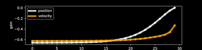
Example
- Setting: UAV hover over to origin \(s_\star = (0,0)\)
- action: thrust right/left, state is pos/vel
- \(F(s_t, a_t) = \begin{bmatrix}1 & 0.1 \\ 0 & 1\end{bmatrix}s_t + \begin{bmatrix}0\\ 1\end{bmatrix}a_t+w_t\)
for \(w_t\) stochastic disturbance - \(c(s,a) = \mathbb E[\mathsf{pos}_t^2 + \lambda_v \mathsf{vel}_t^2 + \lambda_a a_t^2]\)
\(a_t\)
Claim: optimal policy is linear \(\pi_t^\star(s) = \gamma^\mathsf{pos}_t \mathsf{pos}_t + \gamma_t^\mathsf{vel} \mathsf{vel}_t\)
Notice: gains \(\approx\) static for early part of horizon
Example: Safety
The state is position & velocity \(s=[\theta,\omega]\) with \( s_{t+1} = \begin{bmatrix} 1 & 0.1\\ & 1 \end{bmatrix}s_t + \begin{bmatrix} 0\\ 1 \end{bmatrix}a_t\)
- For safety, we must have \(|\theta|\leq 1\)
-
Are trajectories safe as long as \(|\theta_0|<1\)?
- no! Exercise: what is the necessary condition on \(\omega_0\)?
- Suppose we also have an actuation limit \(|a|\leq 0.5\)
- now guaranteeing safety is even more difficult
\(a_t\)
Example: Safety
The state is position & velocity \(s=[\theta,\omega]\) with \( s_{t+1} = \begin{bmatrix} 1 & 0.1\\ & 1 \end{bmatrix}s_t + \begin{bmatrix} 0\\ 1 \end{bmatrix}a_t\)
Goal: stay near origin and be energy efficient
- \(c(s,a) = s^\top \begin{bmatrix} 1 & \\ & 0.5 \end{bmatrix}s + a^2 \)
- Safety constraint \(|\theta|\leq 1\) and actuation limit \(|a|\leq 0.5\)


Example: Infeasibility
The state is position & velocity \(s=[\theta,\omega]\) with \( s_{t+1} = \begin{bmatrix} 1 & 0.1\\ & 1 \end{bmatrix}s_t + \begin{bmatrix} 0\\ 1 \end{bmatrix}a_t\)
Goal: stay near origin and be energy efficient
- Safety constraint \(|\theta|\leq 1\) and actuation limit \(|a|\leq 0.5\)


Definition of Safety
- Fact 2: A short MPC horizon (without proper terminal cost/constraints) can result in loss of stability and safety.
- We define safety in terms of the "safe set" \(\mathcal S_\mathrm{safe}\subseteq \mathcal S\).
-
Definitions:
-
A state \(s\) is safe if \(\mathcal s\in\mathcal S_\mathrm{safe}\).
-
A trajectory of states \((s_0,\dots,s_t)\) is safe if \(\mathcal s_k\in\mathcal S_\mathrm{safe}\) for all \(0\leq k\leq t\).
-
(we can analogously define \(\mathcal A_\mathrm{safe}\subseteq \mathcal A\) and require that \(\mathcal a_k\in\mathcal A_\mathrm{safe}\) for all \(0\leq k\leq t\))
Definition of Safety
- Fact 2: A short MPC horizon (without proper terminal cost/constraints) can result in loss of stability and safety.
- We define safety in terms of the "safe set" \(\mathcal S_\mathrm{safe}\subseteq \mathcal S\).
-
Definitions:
-
A state \(s\) is safe if \(\mathcal s\in\mathcal S_\mathrm{safe}\).
-
A trajectory of states \((s_0,\dots,s_t)\) is safe if \(\mathcal s_k\in\mathcal S_\mathrm{safe}\) for all \(0\leq k\leq t\).
-
A system \(s_{t+1}=F(s_t)\) is safe if some \(\mathcal S_\mathrm{inv}\subseteq \mathcal S_{\mathrm{safe}}\) is invariant, i.e.
- for all \( s\in\mathcal S_\mathrm{inv}\), \( F(s)\in\mathcal S_\mathrm{inv}\)
-
Exercise: Prove that if \(\mathcal S_\mathrm{inv}\) is invariant for dynamics \(F\), then \(s_0\in \mathcal S_\mathrm{inv} \implies s_t\in\mathcal S_\mathrm{inv}\) for all \(t\).
Invariant set for linear dynamics
- Consider stable linear dynamics \(s_{t+1}=Fs_t\).
- Consider the set \( \{s\mid s^\top Ps \leq c\} \) with \(P = \sum_{t=0}^\infty (F^t)^\top F^t\)
-
Claim: This is an invariant set
-
\((Fs)^\top \sum_{t=0}^\infty (F^t)^\top F^t (Fs) \)
-
\(= s^\top \sum_{t=1}^\infty (F^t)^\top F^t s \)
-
\(\leq s^\top \sum_{t=0}^\infty (F^t)^\top F^t s \leq c\)
-

Example: An invariant set for
\(s=[\theta,\omega]\) with \( s_{t+1} = \begin{bmatrix} 0.9 & 0.1\\ & 0.9 \end{bmatrix}s_t \)
Claim: if \(V(s)\) is a Lyapunov function for \(F\) then any sublevel set \(\{V(s)\leq c\}\) is invariant.
Invariant step for stable dynamics
- \(V(F(s))\)
- \(\leq V(s)\)
- \(\leq c\)
Definition: A Lyapunov function \(V:\mathcal S\to \mathbb R\) for \(F\) is continuous and
- (positive definite) \(V(0)=0\) and \(V(0)>0\) for all \(s\in\mathcal S - \{0\}\)
- (decreasing) \(V(F(s)) - V(s) \leq 0\) for all \(s\in\mathcal S\)

- Fact 2: A short MPC horizon (without proper terminal cost/constraints) can result in loss of stability and safety.
- Infeasibility = inability to guarantee safety
- also leads to loss of stability
- States that are initially feasible vs. states that remain feasible
- not different when plan is over \(H=T\)
Infeasibility Problem
- infeasible
- initially feasible
- remain feasible
$$\min_{a_0,\dots,a_{H}} \quad\sum_{k=0}^{H-1} c(s_{k}, a_{k}) +\textcolor{cyan}{ c_H(s_H)}$$
\(\text{s.t.}\quad s_0 = s,\quad s_{k+1} = F(s_{k}, a_{k})\qquad\qquad\)
\(s_k\in\mathcal S_\mathrm{safe},\quad a_k\in\mathcal A_\mathrm{safe},\quad \textcolor{cyan}{s_H\in\mathcal S_H}\)
Terminal cost and constraints
Fact 3: Under the following assumptions, MPC is recursively feasible, i.e. able to guarantee safety indefinitely:
- The origin is uncontrolled fixed pointed \(F(0,0)=0\)
- The terminal constraint is zero \(\mathcal S_H=0\) and the constraints contain the origin \(0\in\mathcal S_\mathrm{safe}\) and \(0\in\mathcal A_\mathrm{safe}\)
Recursive feasibility: feasible at \(s_t\implies\) feasible at \(s_{t+1}\)
Proof:
- \(s_t\) feasible and solution to optimization problem is \(a^\star_{0}, \dots, a^\star_{H-1}\) with corresponding states \(s^\star_{0}, \dots, s^\star_{H}\)
- After applying \(a_t=a^\star_{0}\), state moves to \(s_{t+1} = F(s_t,a_t)\)
- Notice that \(s_{t+1} = s^\star_1\)
- Claim: \(a^\star_{1}, \dots, a^\star_{H-1}, 0\) is now a feasible solution.
- because \(s_{H}^\star=0\) and \(F(0,0)=0\)
- thus corresponding states \(s^\star_{1}, \dots, s^\star_{H}, 0\) satisfy constraints
Recursive Feasibility
$$\min_{a_0,\dots, a_{H}} \quad\sum_{k=0}^{H-1} c(s_{k}, a_{k})\qquad\text{s.t.}\quad s_0 = s_t,\quad s_{k+1} = F(s_{k}, a_{k})$$
\(s_k\in\mathcal S_\mathrm{safe},\quad a_k\in\mathcal A_\mathrm{safe},\quad \textcolor{cyan}{s_H=0}\)

Stability
Fact 4: Under the following assumptions, MPC is provably stabilizing, i.e. $$\tilde F(s) = F(s,\pi_{MPC}(s))~~\text{is stable}$$
- The origin is uncontrolled fixed pointed \(F(0,0)=0\)
- The terminal constraint is zero \(\mathcal S_H=0\) and the constraints contain the origin \(0\in\mathcal S_\mathrm{safe}\) and \(0\in\mathcal A_\mathrm{safe}\)
- The terminal cost is zero \(c_H(s)=0\) and the stage cost \(c(s,a)\) is positive definite, i.e. \(c(s,a)>0\) for all \(s,a\neq 0\) and \(c(0,0)=0\).
$$\min_{a_0,\dots, a_{H}} \quad\sum_{k=0}^{H-1} c(s_{k}, a_{k})\qquad\text{s.t.}\quad s_0 = s_t,\quad s_{k+1} = F(s_{k}, a_{k})$$
\(s_k\in\mathcal S_\mathrm{safe},\quad a_k\in\mathcal A_\mathrm{safe},\quad \textcolor{cyan}{s_H=0}\)
Stability
Fact 4: Under the following assumptions, MPC is provably stabilizing, i.e. $$\tilde F(s) = F(s,\pi_{MPC}(s))~~\text{is stable}$$
-
Proof: Let \(J^\star(s)\) be the objective value for the above with \(s_t=s\). Then the function \(J^\star(s)\) is positive definite and strictly decreasing. Therefore, it is a Lyapunov function for the closed loop dynamics \(F(\cdot, \pi_\mathrm{MPC}(\cdot))\), certifying asymptotic stability.
$$\min_{a_0,\dots, a_{H}} \quad\sum_{k=0}^{H-1} c(s_{k}, a_{k})\qquad\text{s.t.}\quad s_0 = s_t,\quad s_{k+1} = F(s_{k}, a_{k})$$
\(s_k\in\mathcal S_\mathrm{safe},\quad a_k\in\mathcal A_\mathrm{safe},\quad \textcolor{cyan}{s_H=0}\)
- Positive definite:
- if \(s=0\), then optimal actions are \(0\) since \(F(0,0)=0\) and stage cost is positive definite
- if \(s\neq 0\), \(J^\star(s)>0\) since stage cost is positive definite
Stability
- Strictly decreasing: recall \(J^\star (s_t) =\sum_{k=0}^{H-1} c(s^\star_{k}, a^\star_{k}) +0\)
- Let \(J(s; a_0,\dots, a_{H-1})\) be the value of the objective for actions \(a_0,\dots, a_{H-1}\) and \(s_t=s\)
- \(J^\star(s_{t+1}) \leq\) cost of feasible solution starting at \(s_0=F(s_t, a^\star_{0})\)
- \(=J(s_{t+1}; a^\star_1,\dots, a^\star_{H-1}, 0)=\sum_{k=1}^{H-1} c(s^\star_{k}, a^\star_{k}) + c(s^\star_{H}, 0)\)
- \(=\sum_{k=0}^{H-1} c(s^\star_{k}, a^\star_{k}) + \cancel{c(0, 0)} -c(s^\star_{0}, a^\star_{0}) \)
- \(= J^\star (s) -c(s^\star_{0}, a^\star_{0}) < J^\star (s)\)
Terminal cost and constraints
Fact 3 and 4 (general): Under the following assumptions, MPC is recursively feasible, i.e. able to guarantee safety indefinitely, and provably stabilizing, i.e. $$\tilde F(s) = F(s,\pi_{MPC}(s))~~\text{is stable}$$
- The origin is uncontrolled fixed pointed \(F(0,0)=0\)
- The constraints contain the origin and the terminal set is contained in safe set and is control invariant
- Definition: \(\mathcal S_\mathrm{inv}\) is a control invariant set for dynamics \(s_{t+1} = F(s_t, a_t)\) if for all \( s\in\mathcal S_\mathrm{inv}\), there exists an \(a\in\mathcal A_\mathrm{safe}\) such that \( F(s, a)\in\mathcal S_\mathrm{inv}\)
- The costs are positive definite and the terminal cost satisfies \( c_H(s_{t+1}) - c_H(s_t) \leq -c(s_t, a) \) for some \(a\) such that \(s_{t+1} = F(s_{t}, a)\in\mathcal S_H\)
$$\min_{a_0,\dots,a_{H}} \quad\sum_{k=0}^{H-1} c(s_{k}, a_{k}) +\textcolor{cyan}{ c_H(s_H)}$$
\(\text{s.t.}\quad s_0 = s,\quad s_{k+1} = F(s_{k}, a_{k})\qquad\qquad\)
\(s_k\in\mathcal S_\mathrm{safe},\quad a_k\in\mathcal A_\mathrm{safe},\quad \textcolor{cyan}{s_H\in\mathcal S_H}\)
Recursive feasibility: feasible at \(s_t\implies\) feasible at \(s_{t+1}\)
Proof:
- \(s_t\) feasible and solution to optimization problem is \(u^\star_{0}, \dots, u^\star_{H-1}\) with corresponding states \(x^\star_{0}, \dots, x^\star_{H}\)
- After applying \(a_t=u^\star_{0}\), state moves to \(s_{t+1} = F(s_t,a_t)\)
- Notice that \(s_{t+1} = x^\star_1\)
- Claim: there exists a \(u\) such that \(u^\star_{1}, \dots, u^\star_{H-1}, u\) is a feasible solution.
- because \(x_{H}^\star\in\mathcal S_H\) and \(\mathcal S_H\) is control invariant
- thus corresponding states \(x^\star_{1}, \dots, x^\star_{H}, F(x^\star_{H}, u)\) satisfy constraints
Recursive Feasibility
Proof:
\(J^\star(s)\) is positive definite and strictly decreasing. Therefore, the closed loop dynamics \(F(\cdot, \pi_\mathrm{MPC}(\cdot))\) are asymptotically stable.
Stability
- Positive definite: same argument as before
- Strictly decreasing: recall \(J^\star (s_t) =\sum_{k=0}^{H-1} c(x^\star_{k}, u^\star_{k}) +c_H(x_H^\star)\)
- \(J^\star(s_{t+1}) \leq\) cost of feasible solution starting at \(x_0=F(s_t, u^\star_{0})\)
- \(=J(s_{t+1}; u^\star_1,\dots, u^\star_{H-1}, u)\)
- \(=\sum_{k=1}^{H-1} c(x^\star_{k}, u^\star_{k}) + c(x^\star_{H}, u)+c_H(F(x^\star_{H}, u))\)
- \(=\sum_{k=0}^{H-1} c(x^\star_{k}, u^\star_{k})+c_H(x^\star_H)+ c(x^\star_{H}, u)+c_H(F(x^\star_{H}, u))-c_H(x^\star_H) -c(x^\star_{0}, u^\star_{0}) \)
- \(\leq J^\star (s_t) +c(x^\star_{H}, u) - c(x^\star_{H}, u) -c(x^\star_{0}, u^\star_{0}) < J^\star (s_t)\)
- \(J^\star(s_{t+1}) \leq\) cost of feasible solution starting at \(x_0=F(s_t, u^\star_{0})\)
- Terminal constraint not often used (instead: long horizon)
- Soft constraints
- \(x_k+\delta \in\mathcal S_\mathrm{safe}\) and add penalty \(C\|\delta\|_2^2\) to cost
- Stochastic dynamics and disturbances
- consider cost in expectation, but constraints in worst-case or with high probability
- Scenario MPC: use \(K\) disturbance samples to define average/worst-case cost
- Accuracy of costs/dynamics/constraints vs. ease of optimization
- Fast optimization
- Linearization/quadratic approximation, then fast QP solvers
- Sampling based (cross entropy method)
MPC in practice
References: Predictive Control by Borrelli, Bemporad, Morari
Recap
- Safety as constraints/invariance
- Feasibility problem
- Terminal sets and costs
- Proof of feasibility and stability
Next time: control from partial observation
Announcements
- Papers for presentations have been posted: sign up next lecture!
- Fifth assignment due Friday, no assignment over Fall break