21 - Model Predictive Control - ML in Feedback Sys

Model Predictive Control

ML in Feedback Sys #21

Prof Sarah Dean

Reminders/etc

Project midterm update due 11/11
Scribing feedback to come by next week!
Upcoming paper presentations starting next week
Participation includes attending presentations

policy

$\pi_t:\mathcal S\to\mathcal A$

observation

$s_t$

accumulate

$\{(s_t, a_t, c_t)\}$

Safe action in a dynamic world

Goal: select actions $a_t$ to bring environment to low-cost states
while avoiding unsafe states

action

$a_{t}$

$F$

$s$

Motivation for constraints

Recap: Invariant Sets

A set $\mathcal S_\mathrm{inv}$ is invariant under dynamics $s_{t+1} = F(s_t)$ if for all $ s\in\mathcal S_\mathrm{inv}$, $ F(s)\in\mathcal S_\mathrm{inv}$
If $\mathcal S_\mathrm{inv}$ is invariant for dynamics $F$, then $s_0\in \mathcal S_\mathrm{inv} \implies s_t\in\mathcal S_\mathrm{inv}$ for all $t$.
Example: sublevel set of Lyapunov function
- $\{s\mid V(s)\leq c\}$

Recap: Safety

We define safety in terms of the "safe set" $\mathcal S_\mathrm{safe}\subseteq \mathcal S$.
A state $s$ is safe if $\mathcal s\in\mathcal S_\mathrm{safe}$.
A trajectory of states $(s_0,\dots,s_t)$ is safe if $\mathcal s_k\in\mathcal S_\mathrm{safe}$ for all $0\leq k\leq t$.
A system $s_{t+1}=F(s_t)$ is safe if some $\mathcal S_\mathrm{inv}\subseteq \mathcal S_{\mathrm{safe}}$ is invariant and $s_0\in \mathcal S_{\mathrm{safe}}$.

Recap: Constrained Control

$a_t = {\color{Goldenrod} K_t }s_{t}$

$ \underset{\mathbf a }{\min}$ $\displaystyle\sum_{t=0}^T s_t^\top Q s_t + a_t^\top R a_t$

$\text{s.t.}~~s_{t+1} = As_t + Ba_t $

$s_t \in\mathcal S_\mathrm{safe},~~ a_t \in\mathcal A_\mathrm{safe}$

$\begin{bmatrix} \mathbf s\\ \mathbf a\end{bmatrix} = \begin{bmatrix} \mathbf \Phi_s\\ \mathbf \Phi_a\end{bmatrix}\mathbf w $

$\mathbf w = \begin{bmatrix}s_0\\ 0\\ \vdots \\0 \end{bmatrix}$

open loop problem is convex if costs convex, dynamics linear, and $\mathcal S_\mathrm{safe}$ and $\mathcal A_\mathrm{safe}$ are convex
closed-loop linear problem can be reformulated as convex using System Level Synthesis

$ \underset{\color{teal}\mathbf{\Phi}}{\min}$$\left\| \begin{bmatrix}\bar Q^{1/2} &\\& \bar R^{1/2}\end{bmatrix} \begin{bmatrix}\color{teal} \mathbf{\Phi}_s \\ \color{teal} \mathbf{\Phi}_a\end{bmatrix} \mathbf w\right\|_{2}^2$

$\text{s.t.}~~ \begin{bmatrix} I - \mathcal Z \bar A & - \mathcal Z \bar B\end{bmatrix} \begin{bmatrix}\color{teal} \mathbf{\Phi}_s \\ \color{teal} \mathbf{\Phi}_a\end{bmatrix}= I $

$\mathbf \Phi_s\mathbf w \in\mathcal S_\mathrm{safe}^T,~~\mathbf \Phi_a\mathbf w\in\mathcal A_\mathrm{safe}^T$

Recap: Control Barrier Function

Claim: Suppose that for all $t$, the policy satisfies

$C(F(s_t, \pi(s_t)))\leq \gamma C(s_t)$ for some $0\leq \gamma\leq 1$.
Then $\{s\mid C(s)\leq 0\}$ is an invariant set.

$$\pi(s_t) = \arg\min_a \|a - \pi^\star_\mathrm{unc}(s_t)\|_2^2 \quad\text{s.t.}\quad C(F(s_t, a)) \leq \gamma C(s_t) $$

size of $s$

size of $a$

safety constraint

$C(s)=0$

Today: Receding Horizon Control

Instead of optimizing for open loop control...

$ \underset{a_0,\dots,a_T }{\min}$ $\displaystyle\sum_{t=0}^T c(s_t, a_t)$

$\text{s.t.}~~s_0~\text{given},~~s_{t+1} = F(s_t, a_t)$

$s_t \in\mathcal S_\mathrm{safe},~~ a_t \in\mathcal A_\mathrm{safe}$

Observe state
Optimize plan
For $t=0,1,...$
1. Apply planned action

For $t=0,1,\dots$
1. Observe state
2. Optimize plan
3. Apply first planned action

...re-optimize to close the loop

model predicts the trajectory during planning

Also called Model Predictive Control

Figure from slides by Borelli, Jones, Morari

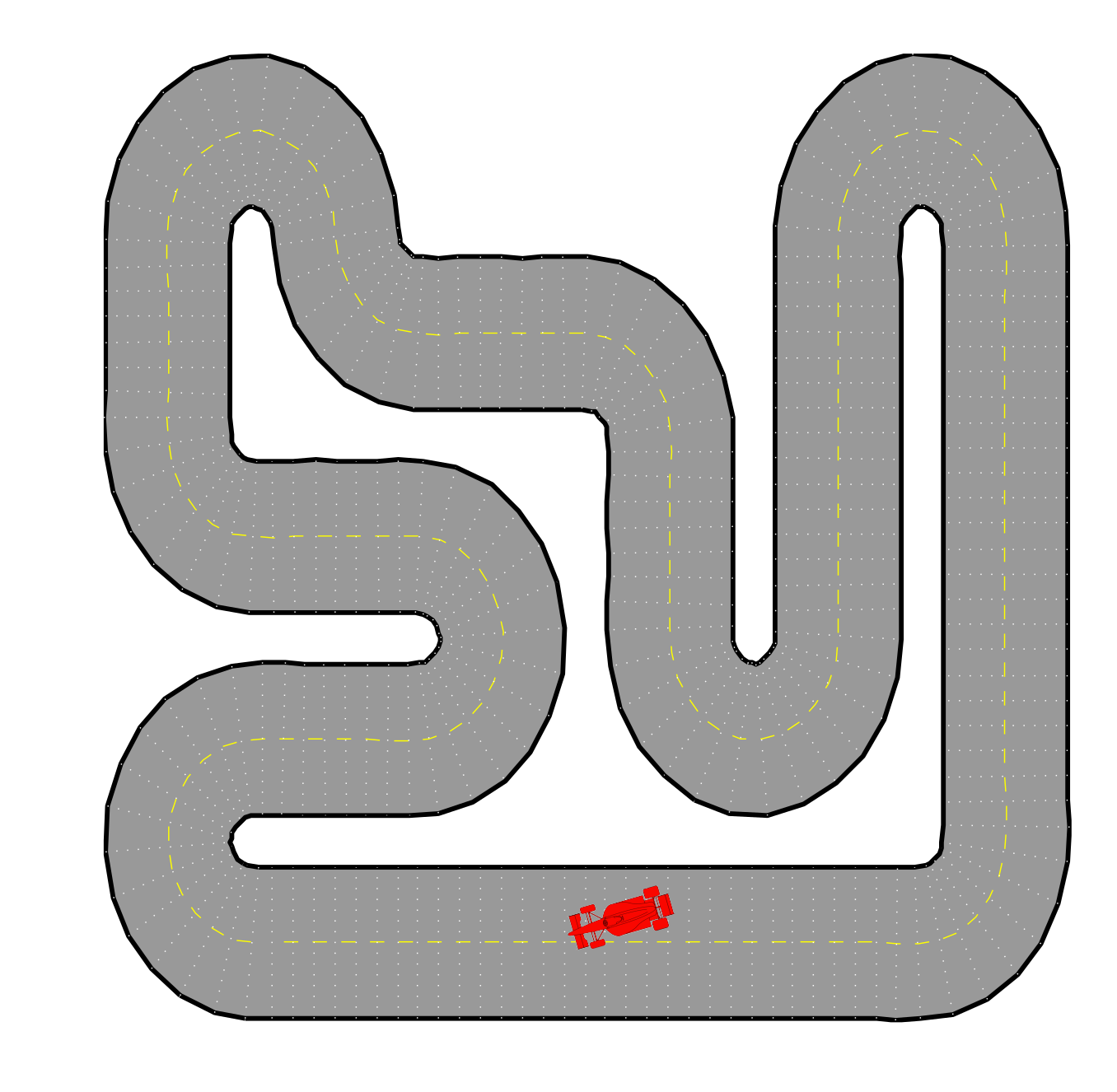
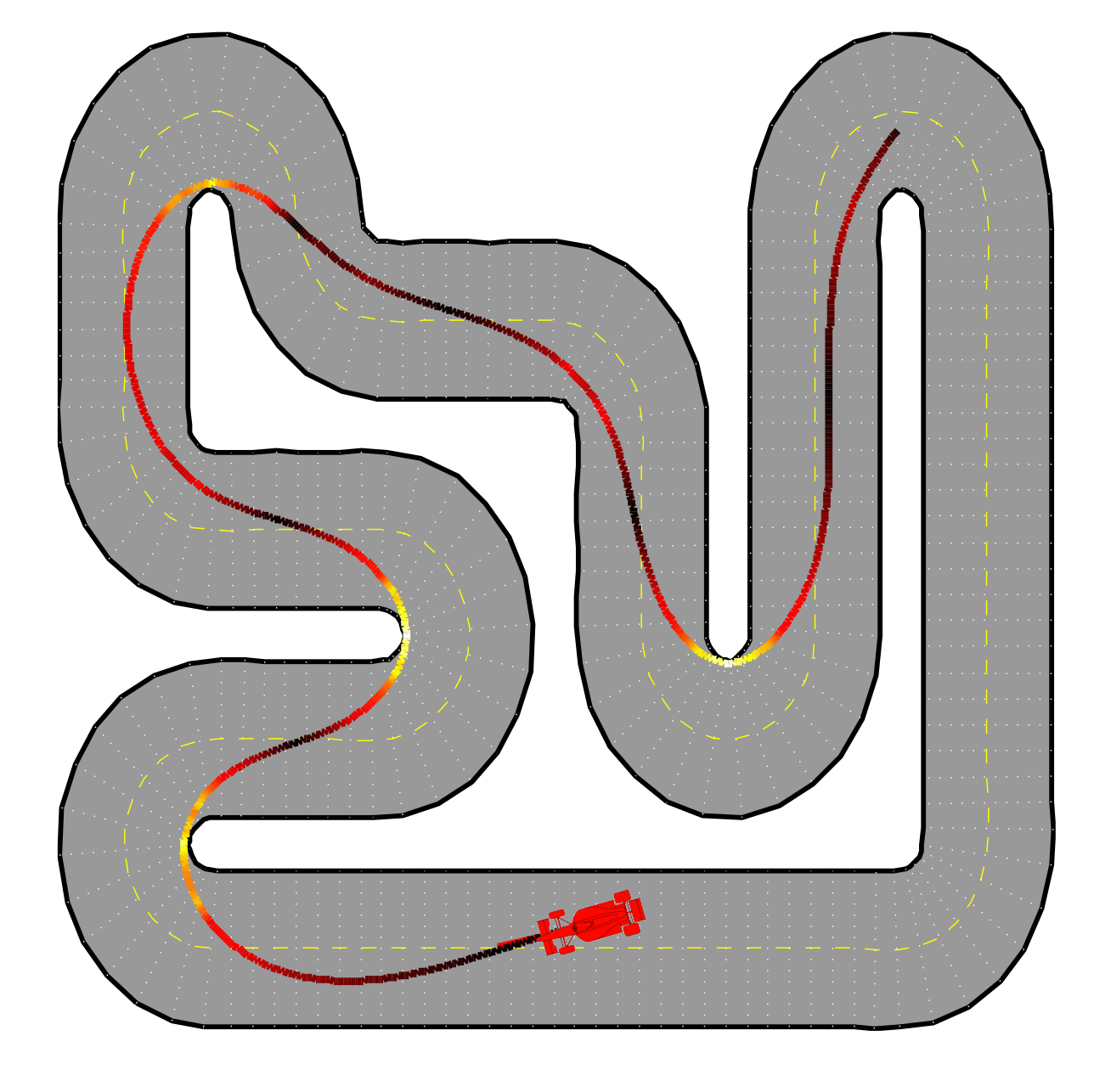
Plan:

minimize lap time
subject to
- car dynamics
- staying within lane
- bounded acceleration

Example: racing

For $t=0,1,\dots$
1. Observe state
2. Optimize plan
3. Apply first planned action

Receding Horizon Leads to Feedback

time

Plan

For $t=0,1,\dots$
1. Observe state
2. Optimize plan
3. Apply first planned action

$a_t$

$F$

$s$

$s_t$

$a_t$

$ \underset{a_0,\dots,a_H }{\min}$ $\displaystyle\sum_{k=0}^H c(s_k, a_k)$

$\text{s.t.}~~s_0~\text{given},~~s_{k+1} = F(s_k, a_k)$

$s_k \in\mathcal S_\mathrm{safe},~~ a_k \in\mathcal A_\mathrm{safe}$

We can:

replan if state $s_{t+1}$ does not evolve as expected (e.g. due to disturbances)
easily incorporate time-varying dynamics, constraints (e.g. obstables), costs (e.g. new incentives)
plan over a shorter horizon than we operate (e.g. $H\leq T$)
- important for realtime computation!

Benefits of Replanning

$\pi(s_t) = u_0^\star(s_t)$

$$\min_{u_0,\dots, u_{H}} \quad\sum_{k=0}^{H} c(x_{k}, u_{k})$$

$\text{s.t.}\quad x_0 = s_t,\quad x_{k+1} = F(x_{k}, u_{k})$

$x_k\in\mathcal S_\mathrm{safe},\quad u_k\in\mathcal A_\mathrm{safe}\quad~~~$

Notation: distinguish real states and actions $s_t$ and $a_t$ from the planned optimization variables $x_k$ and $u_k$.

$[u_0^\star,\dots, u_{H}^\star](s_t) = \arg$

The MPC Policy

$$\min_{u_0,\dots, u_{H}} \quad\sum_{k=0}^{H} c(x_{k}, u_{k})$$

$\text{s.t.}\quad x_0 = s_t,\quad x_{k+1} = F(x_{k}, u_{k})$

$x_k\in\mathcal S_\mathrm{safe},\quad u_k\in\mathcal A_\mathrm{safe}\quad~~~$

Notation: distinguish real states and actions $s_t$ and $a_t$ from the planned optimization variables $x_k$ and $u_k$.

The MPC Policy

$F$

$s$

$s_t$

$a_t = u_0^\star(s_t)$

Example: receding horizon LQR

Infinite Horizon LQR Problem

$$ \min ~~\lim_{T\to\infty}\frac{1}{T}\sum_{t=0}^{T} s_t^\top Qs_t+ a_t^\top Ra_t\quad\\ \text{s.t}\quad s_{t+1} = A s_t+ Ba_t$$

We know that $a^\star_t = \pi^\star(s_t)$ where $\pi^\star(s) = K s$ and

$K = -(R+B^\top PB)^{-1}B^\top QPA$
$P=\mathrm{DARE}(A,B,Q,R)$

Finite LQR Problem

$$ \min ~~\sum_{k=0}^{H} x_k^\top Qx_k + u_k^\top Ru_k \quad \\ \text{s.t}\quad x_0=s,\quad x_{k+1} = A x_k+ Bu_k $$

MPC Policy $a_t = u^\star_0(s_t)$ where
$u^\star_0(s) = K_0s$ and

$K_0 = -(R+B^\top P_{1}B)^{-1}B^\top QP_{1}A$
$P_1=$ backwards DP iteration ($H$ step)

$P = Q+A^\top PA + A^\top PB(R+B^\top PB)^{-1}B^\top PA$
$P_t = Q+A^\top P_{t+1}A + A^\top P_{t+1}B(R+B^\top P_{t+1}B)^{-1}B^\top P_{t+1}A$

Example

The state is position & velocity $s=[\theta,\omega]$ with $ s_{t+1} = \begin{bmatrix} 1 & 0.1\\ & 1 \end{bmatrix}s_t + \begin{bmatrix} 0\\ 1 \end{bmatrix}a_t$

Goal: stay near origin and be energy efficient

$c(s,a) = s^\top \begin{bmatrix} 1 & \\ & 0.5 \end{bmatrix}s + a^2 $
Safety constraint $|\theta|\leq 1$ and actuation limit $|a|\leq 0.5$

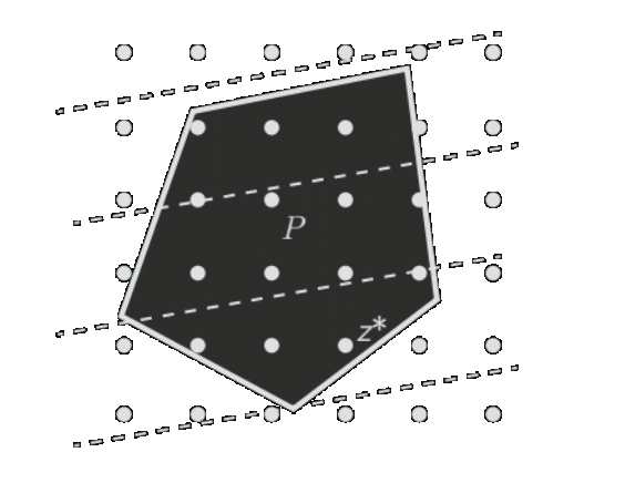
Linear Program (LP): Linear costs and constraints, feasible set is polyhedron. $$\min_z c^\top z~~ \text{s.t.} ~~Gz\leq h,~~Az=b$$
Quadratic Program (QP): Quadratic cost and linear constraints, feasible set is polyhedron. Convex if $P\succeq 0$. $$\min_z z^\top P z+q^\top z~~ \text{s.t.} ~~Gz\leq h,~~Az=b$$

Some types of optimization problems

Figures from slides by Goulart, Borelli

Linear Program (LP): Linear costs and constraints, feasible set is polyhedron. $$\min_z c^\top z~~ \text{s.t.} ~~Gz\leq h,~~Az=b$$
Quadratic Program (QP): Quadratic cost and linear constraints, feasible set is polyhedron. Convex if $P\succeq 0$. $$\min_z z^\top P z+q^\top z~~ \text{s.t.} ~~Gz\leq h,~~Az=b$$
- Nonconvex if $P\nsucceq 0$.

Some types of optimization problems

Figures from slides by Goulart, Borelli

Linear Program (LP): Linear costs and constraints, feasible set is polyhedron. $$\min_z c^\top z~~ \text{s.t.} ~~Gz\leq h,~~Az=b$$
Quadratic Program (QP): Quadratic cost and linear constraints, feasible set is polyhedron. Convex if $P\succeq 0$. $$\min_z z^\top P z+q^\top z~~ \text{s.t.} ~~Gz\leq h,~~Az=b$$
- Nonconvex if $P\nsucceq 0$.
Mixed Integer Linear Program (MILP): LP with discrete constraints. $$\min_z c^\top z~~ \text{s.t.} ~~Gz\leq h,~~Az=b,~~z\in\{0,1\}^n$$

Some types of optimization problems

Figures from slides by Goulart, Borelli

Pros
- Flexibility: any model and any objective
- Guarantees safety by definition*
  - *over planning horizon
Cons
- Computationally demanding
- How to guarantee long term stability/feasibility?

Pros and Cons of MPC

Example: infeasibility

The state is position & velocity $s=[\theta,\omega]$ with $ s_{t+1} = \begin{bmatrix} 1 & 0.1\\ & 1 \end{bmatrix}s_t + \begin{bmatrix} 0\\ 1 \end{bmatrix}a_t$

Goal: stay near origin and be energy efficient

Safety constraint $|\theta|\leq 1$ and actuation limit $|a|\leq 0.5$

Recap

Recap of safety
- invariance, constraints, barrier functions
Receding Horizon Control
MPC Policy and Optimization
Feasibility Problem

References: Predictive Control by Borrelli, Bemporad, Morari

Model Predictive Control

ML in Feedback Sys #21

Reminders/etc

Safe action in a dynamic world

\(F\)

Motivation for constraints

Recap: Invariant Sets

Recap: Safety

Recap: Constrained Control

Recap: Control Barrier Function

Today: Receding Horizon Control

Example: racing

Receding Horizon Leads to Feedback

\(F\)

Benefits of Replanning

The MPC Policy

The MPC Policy

\(F\)

Example: receding horizon LQR

Example

Some types of optimization problems

Some types of optimization problems

Some types of optimization problems

Pros and Cons of MPC

Example: infeasibility

Recap