Set-based and Machine Learning Perspectives on Control-affine Dynamics
Sarah Dean, Cornell
Data-driven nonlinear control
Nonlinear control affine dynamics with state \(\mathbf x\in\mathbb R^n\) and input \(\mathbf u\in\mathbb R^m\)
\(\dot{\mathbf x} = \mathbf f(\mathbf x)+\mathbf g(\mathbf x)\mathbf u\)
\({\mathbf x}_{t+1} = \mathbf f(\mathbf x_t)+\mathbf g(\mathbf x_t)\mathbf u_t\)
functions \(\mathbf f\) and \(\mathbf g\) unknown (or partially unknown)
- Goal: sketch roadmap to sample complexity theory for data-driven nonlinear control
- Three related perspectives:
- Robust control + set-based learning
- Kernel-based learning with approximations
- Sample complexity theory for bilinear systems
This talk:
1. Towards Robust Data-Driven Control Synthesis for Nonlinear Systems with Actuation Uncertainty with Andrew Taylor, Victor Dorobantu, Benjamin Recht, Yisong Yue, Aaron Ames
2. Random Features Approximation for Control-Affine Systems with Kimia Kazemian, Yahya Sattar
3. Finite Sample Identification of Partially Observed Bilinear Dynamical Systems with Yahya Sattar, Yassir Jedra, Maryam Fazel
1. Robust control + set-based learning


Aaron Ames
Ben Recht
Andrew Taylor
Yisong Yue
Victor Dorobantu
Ryan Cosner
Towards Robust Data-Driven Control Synthesis for Nonlinear Systems with Actuation Uncertainty
Setting: nonlinear control
Nonlinear control affine dynamics
\(\mathbf x\in\mathbb R^n, \mathbf u\in\mathbb R^m\)
Goal: design \(\mathbf k\) to certify desired behavior
\(\mathbf u = \mathbf k(\mathbf x)\)
\(\dot{\mathbf x} = \mathbf f(\mathbf x)+\mathbf g(\mathbf x)\mathbf u\)
Approach: Control Certificate Functions
Certficate function \(C:\mathbb{R}^n\to \mathbb R\)
Comparison function \(\alpha:\mathbb{R}\to \mathbb R\)
Control Certificate Condition:
\( \dot C(\mathbf x, \mathbf u) \leq -\alpha(C(\mathbf x)) \)
\(\mathbf k(\mathbf x) \in \{\mathbf u \mid \dot C(\mathbf x, \mathbf u) \leq -\alpha(C(\mathbf x)) \}\)
\(\implies\) desired behavior
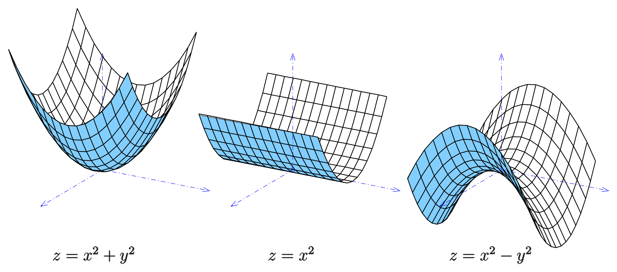
Ex: Control Lyapunov Function (stability)
Ex: Control Barrier Function (safety)
\(C(\mathbf x)\)
\(\mathbf x=0\)
\(\mathbf x\)
\(C(\mathbf x)\leq 0\)
\(\mathbf x\)
Encode control objectives on the basis of instantaneous behavior
Ex: Control Lyapunov Functions (CLF)
Lyapunov function satisfying
\(\alpha_1(\|\mathbf x\|) \leq C(\mathbf x) \leq \alpha_2(\|\mathbf x\|)\)
for \(\alpha_1,\alpha_2\in\mathcal K\)
and comparison function satisfying
\(\alpha \in \mathcal K\)
then if CCF condition can be enforced, stability to the origin guaranteed
CLF-QP:
\(\mathbf k(\mathbf x) = \arg\min_{\mathbf u} \|\mathbf u - \mathbf k_d(\mathbf x)\|_2^2\)
\(\text{s.t.}~~ \dot C(\mathbf x, \mathbf u)\leq -\alpha(C(\mathbf x))\)
(Artstein, 1983; Sontag, 1989; Freeman & Kokotovic, 1996)
(Ames & Powell, 2013)
Given:
\(C(\mathbf x)\)
\(\mathbf x=0\)
\(\mathbf x\)
Ex: Control Barrier Functions (CBF)
then if CCF condition can be enforced, safe set \(\mathcal S\) is guaranteed forward invariant.
(Ames et al., 2017)
barrier function satisfying
\(C(\mathbf x) \leq 0\iff \mathbf x\in\mathcal S\)
and comparison function
\(\alpha \in \mathcal K_e\)
CBF-QP:
\(\mathbf k(\mathbf x) = \arg\min_{\mathbf u} \|\mathbf u - \mathbf k_d(\mathbf x)\|_2^2\)
\(\text{s.t.}~~ \dot C(\mathbf x, \mathbf u)\leq -\alpha(C(\mathbf x))\)
(Ames et al. 2014, 2017)
Given
\(C(\mathbf x)\leq 0\)
\(\mathbf x\)
Example: Feedback Linearizable Systems
- knowing the degree of actuation is sufficient for designing CCF
Control Certificate Condition:
\(K(\mathbf x) = \{\mathbf u \mid \dot C(\mathbf x, \mathbf u) = \nabla C(\mathbf x)^\top (\mathbf f(\mathbf x)+\mathbf g(\mathbf x)\mathbf u) \leq -\alpha(C(\mathbf x)) \}\)
We call \(C\) a Control Certificate Function if \(K(\mathbf x)\) is nonempty for all \(\mathbf x\)
Control Certificate Function
\( L_{\mathbf f} C(\mathbf x)+ L_{\mathbf g}C(\mathbf x)\mathbf u\)
(Dimitrova & Majumdar, 2014)
(Boffi et al., 2020)
Designing CCFs is nontrivial---but not the focus today
Problem setting: uncertain dynamics
Nonlinear control affine dynamics: \(\dot{\mathbf x} = \mathbf f(\mathbf x)+\mathbf g(\mathbf x)\mathbf u\)
State observation
Unknown dynamics \(\mathbf f\) and \(\mathbf g\)
Assumptions:
- \(\mathbf f\) and \(\mathbf g\) are Lipshitz and we know upper bounds on the constants: \(\mathcal L_{\mathbf f}\) and \(\mathcal L_{\mathbf g}\)
-
Access to data \(\{(\dot{\mathbf x}_i, \mathbf x_i, \mathbf u_i)\}_{i=1}^N\)
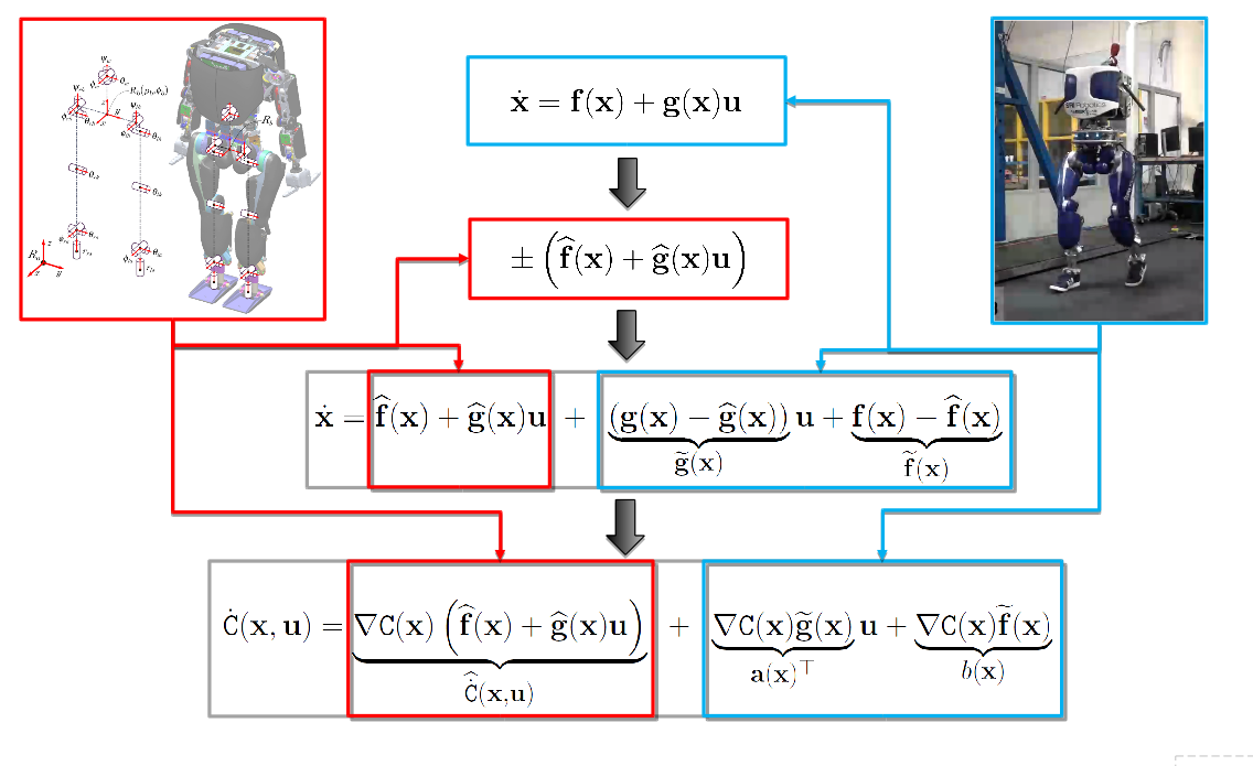
To robustify CCF, characterize all possible \(\mathbf f\) and \(\mathbf g\) consistent with data \(\{(\dot{\mathbf x}_i, \mathbf x_i, \mathbf u_i)\}_{i=1}^N\)
Data-driven uncertainty set
Pointwise uncertainty set:
\(\mathcal U_i(\mathbf x) = \{(\mathbf a, \mathbf B) \mid \|\mathbf a + \mathbf B \mathbf u_i-\dot{\mathbf x}_i\| \leq (\mathcal L_{\mathbf f} + \mathcal L_{\mathbf g}\|\mathbf u_i\|)\|\mathbf x - \mathbf x_i\|\}\)
We can guarantee that \(\mathbf f(\mathbf x), \mathbf g(\mathbf x) \in \mathcal U_i(\mathbf x)\)
\( \|\mathbf f(\mathbf x)+\mathbf g(\mathbf x) \mathbf u_i -\dot{\mathbf x}_i \|\leq \|\mathbf f(\mathbf x)-\mathbf f(\mathbf x_i)\|+\|\mathbf g(\mathbf x) \mathbf -\mathbf g(\mathbf x_i) \|\|\mathbf u_i\|\)
\(\mathbf f(\mathbf x)+\mathbf g(\mathbf x) \mathbf u_i = \dot{\mathbf x}_i + (\mathbf f(\mathbf x)-\mathbf f(\mathbf x_i))+(\mathbf g(\mathbf x) \mathbf -\mathbf g(\mathbf x_i) )\mathbf u_i\)
\(\mathbf f(\mathbf x), \mathbf g(\mathbf x) \in \cap_{i=1}^N \mathcal U_i(\mathbf x)= \mathcal U(\mathbf x)\)

Uncertainty Set Visualization
\(\begin{bmatrix} u_1\\ 1 \end{bmatrix}\)
\(\left |\begin{bmatrix} u_i\\1 \end{bmatrix}^\top\begin{bmatrix} b \\ a \end{bmatrix} - \dot{ x}_i \right|\leq \mathcal L_i |x-x_i| \)
\(\begin{bmatrix} g(x) \\f(x)\end{bmatrix}\)
\(\begin{bmatrix} u_2\\ 1 \end{bmatrix}\)
'Slice' between two planes
Width determined by \(|x-x_i|\)
Direction determined by \(u_i\)
\(\begin{bmatrix} g(x_1) \\f(x_1)\end{bmatrix}\)
Robust CCF Optimization Problem
R-OP:
\(\mathbf k_\mathrm{rob}(\mathbf x)=\argmin\limits_{\mathbf u \in \mathbb{R}^m} \| \mathbf u - \mathbf k_d(\widehat{\mathbf x}) \|\)
\(~~~~~~~~~\text{s.t.}~~\nabla C(\mathbf x)^\top (\mathbf a + \mathbf B\mathbf u)\leq -\alpha(C(\mathbf x))\)
\(~~~~~~~~~~~~~~~~\text{for all}~(\mathbf a, \mathbf B)\in\mathcal U(\mathbf x)\)
Main Result: R-OP is convex, equivalent to a SOCP with \(n\times N\) additional optimization variables, and guarantees that
\(\dot{C}(\mathbf x,\mathbf k_\mathrm{rob}(\mathbf x)) \leq -\alpha C(\mathbf x)\)
Robust Feasibility
Feasibility Result: R-OP is feasible at \(\mathbf x\)
if and only if
\(( -\gamma\alpha(C(\mathbf x)), \mathbf 0)\notin \nabla C(x)^\top \mathcal U(\mathbf x)\) for all \(\gamma>1\)
open loop unsafe/unstable
\(\mathbb R^m\)
\(\mathbb R\)
\(\begin{bmatrix} \nabla C(\mathbf x)^\top \mathbf g(\mathbf x) \\\nabla C(\mathbf x)^\top \mathbf f(\mathbf x)\end{bmatrix}\)
\(\mathcal U_C(\mathbf x) \)
\(-\alpha(C(\mathbf x))\)
R-OP:
\(\mathbf k_\mathrm{rob}(\mathbf x)=\argmin\limits_{\mathbf u \in \mathbb{R}^m} \| \mathbf u - \mathbf k_d(\widehat{\mathbf x}) \|\)
\(~~~~~~~~~\text{s.t.}~~\nabla C(\mathbf x)^\top (\mathbf a + \mathbf B\mathbf u)\leq -\alpha(C(\mathbf x))\)
\(~~~~~~~~~~~~~~~~\text{for all}~(\mathbf a, \mathbf B)\in\mathcal U(\mathbf x)\)
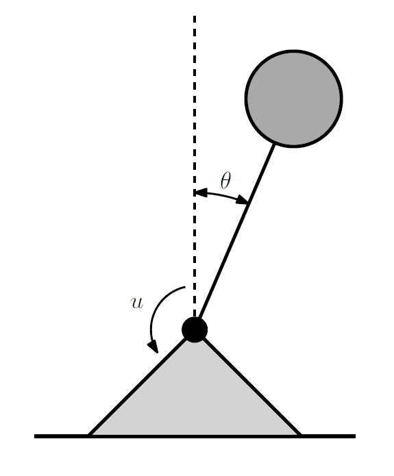
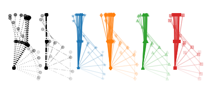
Simulation
-
Inverted pendulum with input gain attenuation \(\propto e^{-\theta^2}\)
-
Stability (CLF) and safety (CBF)
-
Data: densely sampled states, both dense and sparsely sampled inputs
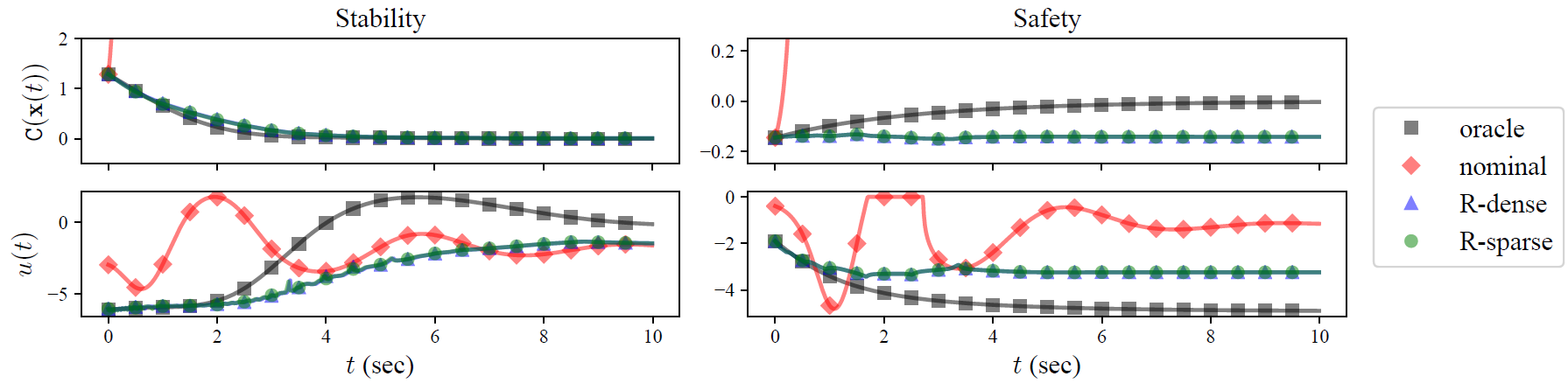
nominal controller unsafe/unstable
data-driven controllers safe/stable
sparse and dense controllers nearly identical
Episodic Learning
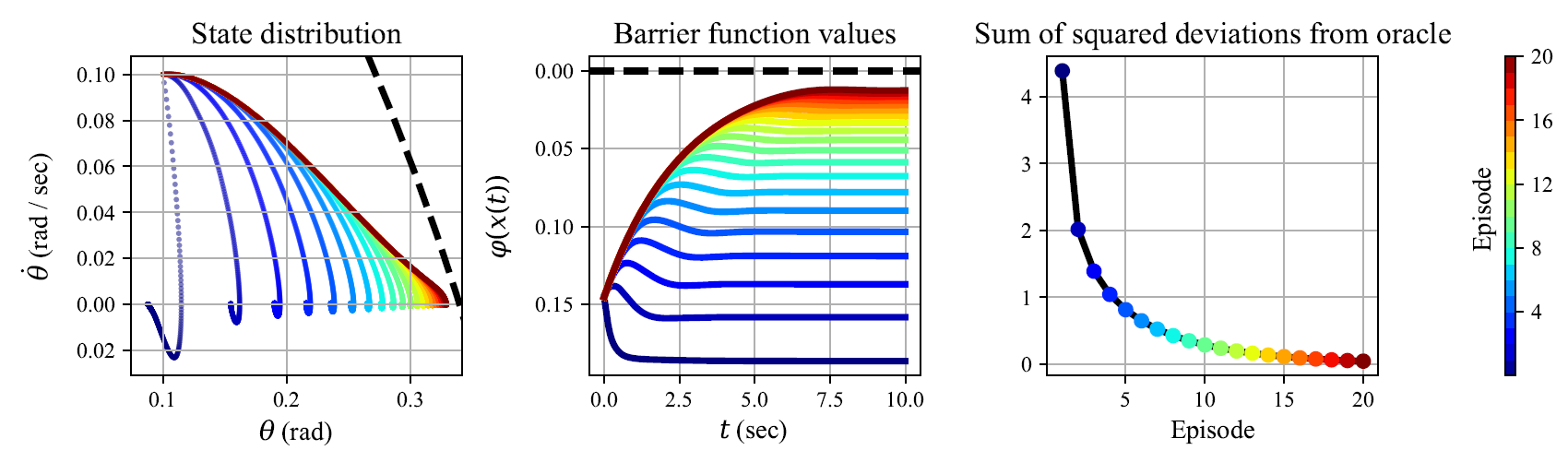
Append data from each episode and restart trajectory
Open Questions
- Control: Design of feasible robust CCFs
- (or other nonlinear control strategy)
- Modelling: Efficiency
- pointwise SOCP complexity is polynomial (cubic/quartic) in \(nN\)
- Data: Sample Complexity
- intuition: dense state coverage (exponential in dimension), linear control coverage (linear in dimension)
- instead: episodic perspective?
2. Kernel-based learning with approx.
Random Features Approximation for Control-Affine Systems
Yahya Sattar
Kimia Kazemian

Setting: control-affine models
Data \(\{(z_i, \mathbf x_i, \mathbf u_i)\}_{i=1}^N\) where \(z_i\) is posited to have a control-affine dependence on \(\mathbf x_i, \mathbf u_i\)
Ex - modelling \(j^{th}\) state coordinate
of control affine dynamics $$z_i = [\dot{\mathbf x}_i]_j = f_j(\mathbf x_i) + \mathbf g_j(\mathbf x_i)^\top \mathbf u_i$$
Ex - modelling CCF $$z_i = \dot C(\mathbf x_i,\mathbf u_i) = \nabla C(\mathbf x_i)^\top \mathbf f(\mathbf x_i) +\nabla C(\mathbf x_i)^\top \mathbf g(\mathbf x_i)^\top\mathbf u_i$$

Approach: kernel regression and random feature approximation
Background: Kernel Regression
Given a kernel function, for generic data \(\{(z_i, \mathbf s_i)\}_{i=1}^N\), kernel ridge regression gives the predictor
Rigorous pointwise uncertainty quantification \(\sigma(\mathbf s)\) (Gaussian process)
Many kernel function are expressive enough to approximate continuous functions arbitrarily well
\(h(\mathbf s) = \mathbf k(\mathbf s)^\top (\mathbf K+\lambda \mathbf I_N)^{-1}\mathbf z \)
where \(\mathbf k(\mathbf s)_i = k(\mathbf s, \mathbf s_i),\quad \mathbf K_{ij} = k(\mathbf s_i,\mathbf s_j),\quad i,j=1,...,N\)
Background: Random Features
\(h_k(\mathbf s) = \mathbf k(\mathbf s)^\top (\mathbf K+\lambda \mathbf I_N)^{-1}\mathbf z \)
training requires \(N\times N\) matrix inversion (cubic)
prediction requires \(N\) inner products (linear)
Strategy: replace kernel function with inner products of random basis \(\mathbf \phi:\mathbb R^n\to R^D\) so \(k(\mathbf s, \mathbf s') \leftarrow \boldsymbol \psi(\mathbf s) ^\top \boldsymbol \psi(\mathbf s') \)
\(h_\psi(\mathbf s) = \boldsymbol \psi (\mathbf s)^\top (\Psi^\top \Psi+\lambda \mathbf I_D)^{-1} \Psi^\top \mathbf z \)
where \(\Psi = \begin{bmatrix} \boldsymbol \psi(\mathbf s_1) ^\top \\ \vdots \\ \boldsymbol \psi(\mathbf s_N) ^\top \end{bmatrix} \) has dimension \(N\times D\)
For large enough \(D\) and appropriately defined \(\boldsymbol \psi\), \(h_\psi\approx h_k\)
Background: Random Features
\(h_k(\mathbf s) = \mathbf k(\mathbf s)^\top (\mathbf K+\lambda \mathbf I_N)^{-1}\mathbf z \)
training requires \(N\times N\) matrix inversion (cubic)
prediction requires \(N\) inner products (linear)
Strategy: replace kernel function with inner products of random basis \(\boldsymbol \psi:\mathbb R^n\to \mathbb R^D\) so \(k(\mathbf s, \mathbf s') \leftarrow \boldsymbol \psi(\mathbf s) ^\top \boldsymbol \psi(\mathbf s') \)
\(h_\psi(\mathbf s) = \boldsymbol \psi (\mathbf s)^\top (\Psi^\top \Psi+\lambda \mathbf I_D)^{-1} \Psi^\top \mathbf z \)
training is now \(O(ND^2+D^3)\)
prediction is \(O(D)\)
For large enough \(D\) and appropriately defined \(\boldsymbol \psi\), \(h_\psi\approx h_k\)
\(\boldsymbol\theta\)

*Ali Rahimi and Benjamin Recht. Random features for large-scale kernel machines. In Proceedings of the 20th International Conference on Neural Information Processing Systems, NIPS’07
Define \( \zeta_\vartheta(s)=e^{-i2\pi\vartheta^\top s}\), then observe:
Euler's formula: \(e^{ix}= \cos x+ i \sin x\)
Background: Random Features
Strategy: replace kernel function with inner products of random basis \(k(\mathbf s, \mathbf s') \leftarrow \boldsymbol \psi(\mathbf s) ^\top \boldsymbol \psi(\mathbf s') \)
Example: Gaussian (RBF) Kernel
Compound kernels and features
Individual kernels/feature functions (each input dimension) $$k_j(\mathbf x,\mathbf x),\quad \boldsymbol \psi_j(\mathbf {x}),\quad j=1,...,m+1$$
Affine Dot Product (ADP) Basis $$\boldsymbol \phi_c(\mathbf x,\mathbf u)=\begin{bmatrix} u_1\boldsymbol \psi_1(\mathbf x) \\ \dots \\ u_{m}\boldsymbol \psi_{m} (\mathbf x) \\ \boldsymbol \psi_{m+1}(\mathbf x) \end{bmatrix} \in \mathbb R^{D(m+1)}$$
Affine Dense (AD) Basis $$\boldsymbol \phi_d(\mathbf x,\mathbf u)=\begin{bmatrix} \boldsymbol \psi_1(\mathbf x)^\top \\ \dots \\ \boldsymbol \psi_{m} (\mathbf x)^\top \\ \boldsymbol \psi_{m+1}(\mathbf x)^\top \end{bmatrix}^\top \begin{bmatrix} \mathbf u \\ 1 \end{bmatrix} \in \mathbb R^D$$
corresponds to ADP compound kernel defined by \(k_1,...,k_{m+1}\) (Castaneda et al., 2020)
corresponds to AD compound kernel defined by \(k_1,...,k_{m+1}\) (novel)
Compound kernels and features
Individual kernels/feature functions (each input dimension) $$k_j(\mathbf x,\mathbf x),\quad \boldsymbol \psi_j(\mathbf {x}),\quad j=1,...,m+1$$
Affine Dot Product (ADP) Kernel $$k_c(\mathbf {x,u,x', u'})=\sum_{j=1}^m u_j u'_j k_j(\mathbf x,\mathbf x') +k_{m+1}(\mathbf x,\mathbf x')$$
Affine Dense (AD) Kernel $$k_d(\mathbf {x,u,x', u'})=\sum_{j=1}^m u_j u'_j k_j(\mathbf x,\mathbf x') + \sum_{\ell=1}^m \sum_{j\neq \ell }^m u_j u'_\ell k_j(\mathbf x,0)k_\ell(0,\mathbf x') +k_{m+1}(\mathbf x,\mathbf x')$$
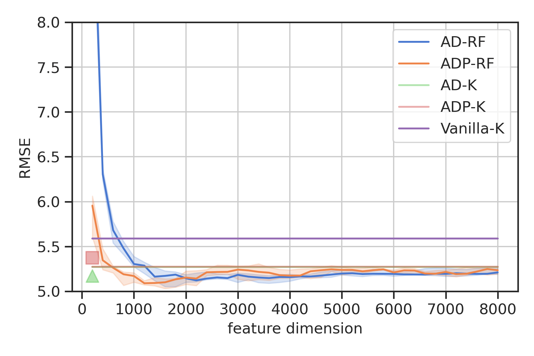
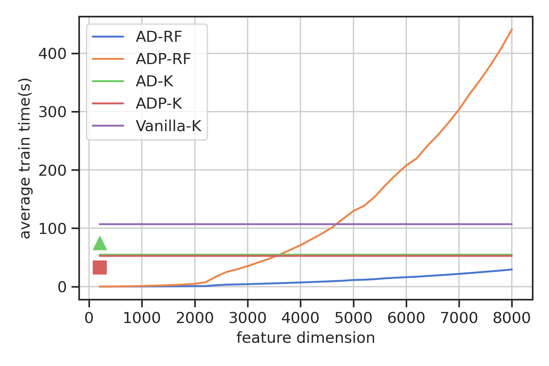
AD-K
time: \(\quad O(N^3)\)
space: \(\quad O(N^2) \)
ADP-RF
time: \(\quad O(N(D(m+1))^2)\)
space: \(\quad O(ND(m+1)) \)
AD-RF
time: \(\quad O(ND^2)\)
space: \(\quad O(ND) \)
Vanilla K
time: \(\quad O((N+m)^3)\)
space: \( \quad O((n+m)^2) \)
ADP-K
time: \( \quad O(N^3)\)
space: \(\quad O(N^2) \)
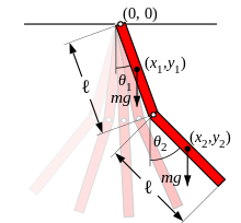
Simulation
-
Double inverted pendulum (\(n=4,m=2)\)
-
Goal: Swing up (CLF)
-
Data: \(N=8.8\)k collected with nominal
-
RBF kernels and random Fourier features
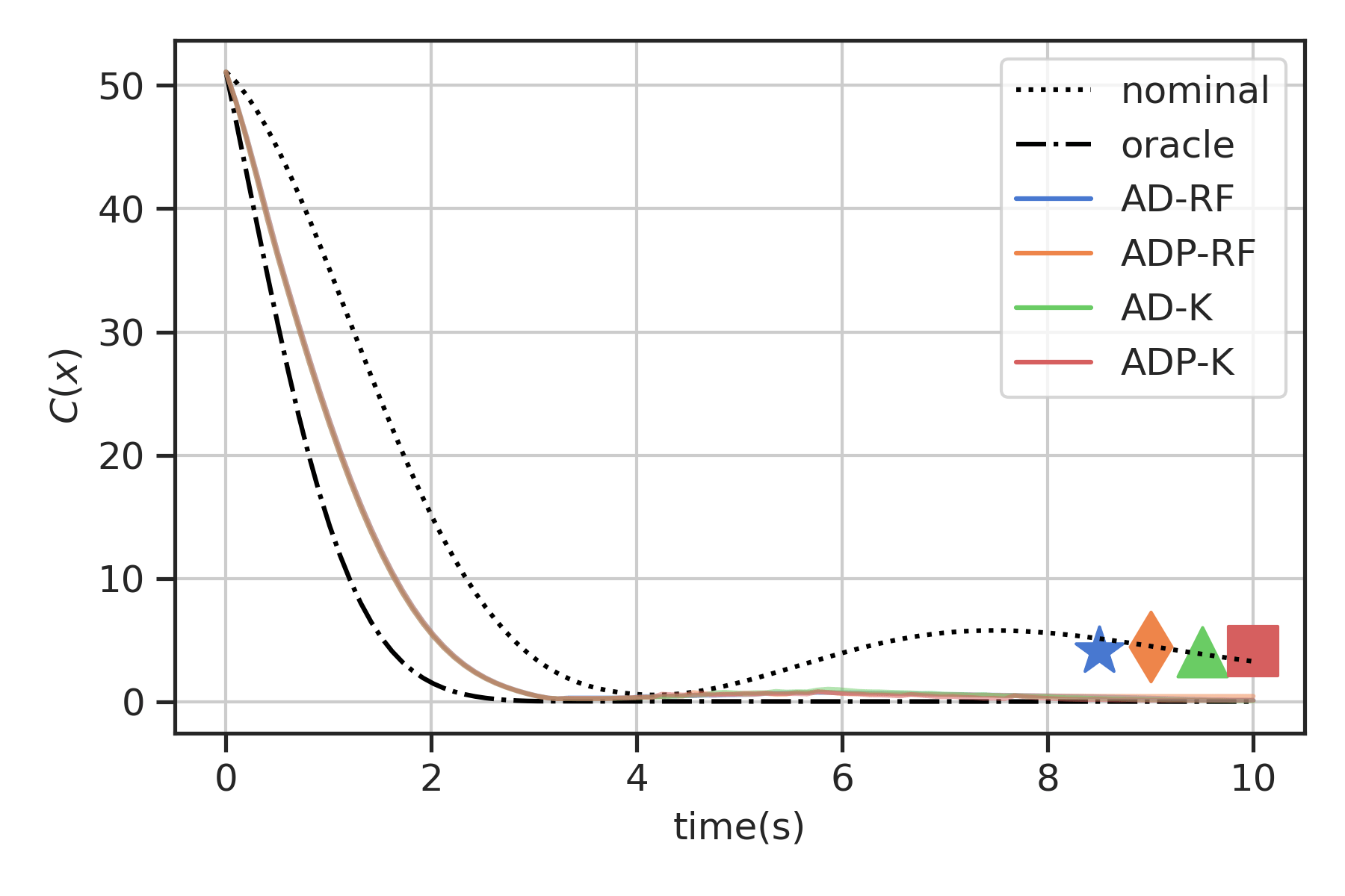
Simulation
-
Double inverted pendulum (\(n=4,m=2)\)
-
Goal: Swing up (CLF)
-
Data: \(N=1.8\)k nominal (subsampled) \(+\) \(1\)k episodic data collection
-
Basis \(D=N/5\)
Open Questions
- Modelling: Efficiency
- Prune data (adaptively?)
- Fast linear algebra
- Data: Sample Complexity
- Kernel intuition: exponential in (state) dimension
- Alternatively, notice that the (partial) model outputs are bilinear in transformed state:
\(h_\psi(\mathbf x,\mathbf u) =\boldsymbol \theta^\top \boldsymbol \psi_{1:m+1}(\mathbf x)^\top \begin{bmatrix} \mathbf u \\ 1 \end{bmatrix}\)
3. Sample complexity theory for bilinear systems
Finite Sample Identification of Partially Observed Bilinear Dynamical Systems
Yahya Sattar
Yassir Jedra
Maryam Fazel


Setting: Bilinear Dynamical Systems (BLDS)
Can approximate control-affine dynamics via Carleman linearization (Kowalski & Steeb, 1991) or Koopman transform (Goswami & Paley, 2017)
Where:
- \( \mathbf x_t \in \mathbb{R}^n \): State
- \( \mathbf u_t \in \mathbb{R}^m \): Input
- \( \mathbf y_t \in \mathbb{R}^p \): Output
- \( \mathbf w_t \in \mathbb{R}^n \): Process noise
- \( \mathbf z_t \in \mathbb{R}^p \): Measurement noise
- \( A_0, A_1, ..., A_m \in \mathbb{R}^{n \times n} \), \( B \in \mathbb{R}^{n \times m} \), \( C \in \mathbb{R}^{p \times n} \), \( D \in \mathbb{R}^{p \times m} \)
$$\mathbf x_{t+1} = (\mathbf u_t \circ \mathbf A)\mathbf x_t + B \mathbf u_t + \mathbf w_t \\ \mathbf y_t = C \mathbf x_t + D \mathbf u_t + \mathbf z_t\qquad\quad $$
where we define
$$\mathbf u_t \circ \mathbf A = A_0 + \sum_{k=1}^m (\mathbf u_t)_k A_k$$
Setting: Bilinear Dynamical Systems (BLDS)
Can approximate control-affine dynamics via Carleman linearization (Kowalski & Steeb, 1991) or Koopman transform (Goswami & Paley, 2017)
$$\mathbf x_{t+1} = (\mathbf u_t \circ \mathbf A)\mathbf x_t + B \mathbf u_t + \mathbf w_t \\ \mathbf y_t = C \mathbf x_t + D \mathbf u_t + \mathbf z_t\qquad\quad $$
where we define
$$\mathbf u_t \circ \mathbf A = A_0 + \sum_{k=1}^m (\mathbf u_t)_k A_k$$
- Suppose \( A_0, A_1, ..., A_m , B,C ,D \) unknown
- Approach: learn input/output map with least squares
Output in terms of past \(L\) inputs:
$$\mathbf y_t = \sum_{\ell=1}^L C \left( \prod_{i=1}^{\ell-1} (\mathbf u_{t-i} \circ \mathbf A) \right) B \mathbf u_{t-\ell} + D \mathbf u_t + \text{noise and error} $$
Truncation error:
$$C \left( \prod_{\ell=1}^L (\mathbf u_{t-\ell} \circ \mathbf A) \right) \mathbf x_{t-L} $$
Process and measurement noise: $$\sum_{\ell=1}^L C \left( \prod_{i=1}^{\ell-1} (\mathbf u_{t-i} \circ \mathbf A) \right) \mathbf w_{t-\ell} + \mathbf v_t $$
Input/output map
\(t\)
\(L\)
\(\underbrace{\qquad\qquad}\)
inputs
outputs
time
Learning the Markov-like Parameters
Define:
- \( \bar{u}_t = [1, u_t] \)
- \( \tilde{u}t = u_t, u{t-1}, \bar{u}{t-1} \otimes u{t-2}, \ldots \)
- \( \tilde{w}t = z_t, w{t-1}, \ldots \)
Then:
$$y_t = \tilde{G} \tilde{u}_t + F \tilde{w}_t + \epsilon_t $$
Output in terms of past \(L\) inputs:
$$\mathbf y_t = \sum_{\ell=1}^L C \left( \prod_{i=1}^{\ell-1} (\mathbf u_{t-i} \circ \mathbf A) \right) B \mathbf u_{t-\ell} + D \mathbf u_t + \text{noise and error} $$
Input/output map
\(t\)
\(L\)
\(\underbrace{\qquad\qquad}\)
inputs
outputs
time
$$\mathbf y_t = {G} \tilde{\mathbf u}_t + \text{noise and error} $$
- Define $$\bar{\mathbf u} = \begin{bmatrix}1 & \mathbf u^\top \end{bmatrix}^\top $$
- $$\tilde{\mathbf u}_t = \begin{bmatrix} \mathbf u_t \\ \mathbf u_{t-1} \\ \bar{\mathbf u}_{t-1} \otimes \mathbf u_{t-2} \\ \bar{\mathbf u}_{t-1} \otimes \bar{\mathbf u}_{t-2} \otimes \mathbf u_{t-3}\\ \vdots \\ \bar{\mathbf u}_{t-1} \otimes \bar{\mathbf u}_{t-2} \otimes \dots \otimes \mathbf u_{t-L} \end{bmatrix} \in \mathbb R^{\tilde m}$$ where \( \tilde m={(m+1)^L+m-1}\)
- Define \(\mathcal A\) as the set of matrix monomials in \(A_0,...,A_m\) up to degree \(L\) $$G = \mathsf{concat}(D, CMD | M\in\mathcal A) \in\mathbb R^{p\times \tilde m}$$ where \( \tilde m={(m+1)^L+m-1}\)
- $$\bar{\mathbf u} = \begin{bmatrix}1 & \mathbf u^\top \end{bmatrix}^\top $$
- $$\tilde{\mathbf u}_t = \begin{bmatrix} \mathbf u_t \\ \mathbf u_{t-1} \\ \bar{\mathbf u}_{t-1} \otimes \mathbf u_{t-2} \\ \bar{\mathbf u}_{t-1} \otimes \bar{\mathbf u}_{t-2} \otimes \mathbf u_{t-3}\\ \vdots \\ \bar{\mathbf u}_{t-1} \otimes \bar{\mathbf u}_{t-2} \otimes \dots \otimes \mathbf u_{t-L} \end{bmatrix} \in \mathbb R^{\tilde m}$$
Least squares estimation
$$\mathbf y_t = {G} \tilde{\mathbf u}_t + \text{noise and error} $$
$$\hat{G} := \left( \sum_{t=L}^T \mathbf y_t \tilde{\mathbf u}_t^\top \right) \left( \sum_{t=L}^T \tilde{\mathbf u}_t \tilde{\mathbf u}_t^\top \right)^\dagger $$
Theorem (Informal):
Under i.i.d. uniform inputs, stability, and sub-Gaussian noise assumptions, with high probability:
$$\|\hat{G} - G\| \lesssim \sqrt{\frac{m^2 L(m+1)^{L+1} (\log(L/\delta)+p+nL)}{(T-L)(1-\rho)}} $$
- Stability is input-dependent
- Determined by matrix products \(\mathbf u_t \circ \mathbf A\)
- Define: Joint spectral radius for a set of matrices \(\mathcal M\) $$\rho(\mathcal{M}) = \lim_{k\to\infty}\sup_{M_1,...,M_k\in\mathcal M} \|M_1M_2...M_k\|^{1/k}$$ and \(\varphi(\mathcal M, \rho) = \sup_{k\geq1,M_1,...,M_k\in\mathcal M} \frac{1}{\rho^k}\|M_1M_2...M_k\|\)
- Define: BLDS is \((\mathcal U,\kappa,\rho)\)-stable if \(\rho(\mathcal M)\leq \rho<1\) and \(\varphi(\mathcal M, \rho) \leq \kappa\) for \(\mathcal M = \{\mathbf u\circ \mathbf A | u\in\mathcal U\}\)
Stability of BLDS
Assumptions
- Inputs are chosen uniformly at random from sphere \( \sqrt{m} \mathcal S^{m-1}\)
- BLDS is \(( \sqrt{m} \mathcal S^{m-1},\rho,\kappa)\) stable
- Process and measurement noise are sub-Gaussian
Proof Ingredients
1. Persistence of Excitation
$$\lambda_{\min} \left( \sum_{t=L}^T \tilde{u}_t \tilde{u}_t^\top \right) \geq \frac{T-L}{4} $$
- Necessary for consistent estimation
- Requires isotropic inputs
2. Bounded Effect of Noise
- Multiplier process
- Requires independent noise
3. Truncation Bias
- Requires stability
- Unlike in LTI systems, also requires independent noise
Theorem (Informal):
Under i.i.d. uniform inputs, stability, and sub-Gaussian noise assumptions, with high probability:
$$\|\hat{G} - G\| \lesssim \sqrt{\frac{m^2 L(m+1)^{L+1} (\log(L/\delta)+p+nL)}{(T-L)(1-\rho)}} $$
Open Questions
- Can we relax stability assumption?
- Can we estimate reduced number of parameters?
- Can we reduce or remove dependence on state dimension?
- Can we formalize control-affine model connections?
- Can we combine with control for end-to-end performance guarantee?
- Towards Robust Data-Driven Control Synthesis for Nonlinear Systems with Actuation Uncertainty (https://arxiv.org/abs/2011.10730) with Andrew Taylor, Victor Dorobantu, Benjamin Recht, Yisong Yue, Aaron Ames
- Random Features Approximation for Control-Affine Systems (https://arxiv.org/abs/2406.06514) with Kimia Kazemian, Yahya Sattar
- Finite Sample Identification of Partially Observed Bilinear Dynamical Systems (https://arxiv.org/abs/2501.07652) with Yahya Sattar, Yassir Jedra, Maryam Fazel