Recovering and Steering Belief States in Partially Observed Systems

Sarah Dean, Cornell University

CS Colloquium at RPI, September 2026

"Next token prediction"

Auto-regressive architectures trained with next element prediction loss have had great success in many domains

$$ (o_0, o_1, o_2, o_3, o_4, o_5 ..., o_t) \rightarrow o_{t+1} $$

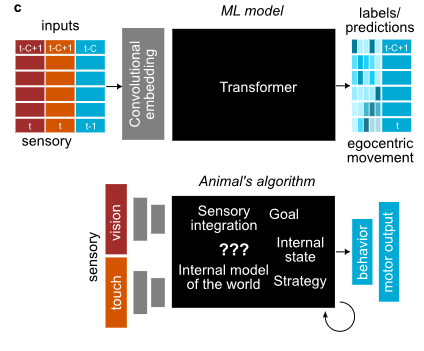
Eyjolfsdottir & Branson, Agent-Centric Animal Pose Forecasting

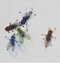
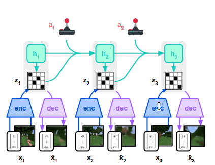
Haffner et al., Mastering Diverse Domains through World Models

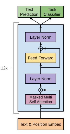
Radford et al., Improving Language Understanding by Generative Pre-Training

natural language

robotics

biology

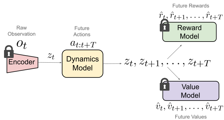
Many researchers are interested in intermediate network activations, whether for use in downstream tasks or for scientific understanding

Inside the black box...

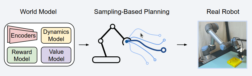
Levy et al., Simulation Distillation: Pretraining World Models
in Simulation for Rapid Real-World Adaptation

Eyjolfsdottir & Branson, Agent-Centric Animal Pose Forecasting

robotics

biology

Outline:

1. Recovering Latent States

2. Control from Partial Observation

filter

controller

$y$

$u$

system

$x$

Partially observed stochastic dynamical system

$$ x_{t+1} = f(x_t,u_t,w_t),\quad y_t = g(x_t, v_t) $$

Inputs $u_t$ and outputs $y_t$ are observed
States $x_t$, process noise $w_t$, measurement
noise $v_t$ are unobserved

Setting: stochastic dynamics

ex: UAV

$x$

$f$

$g$

$w$

$v$

Irreducible uncertainty in state is described by the posterior distribution

$$P(x_t | y_0, u_0, y_1, u_1,...,y_t) $$

$u$

$y$

$$x_0\sim \mathcal D_0, w_t\sim \mathcal D_w, v_t\sim \mathcal D_v$$

Computing this posterior is called filtering $$P(x_t|y_0,...,y_t) \propto P(x_{t-1}|y_0,...,y_{t-1}) P(x_t|x_{t-1} , u_t, y_{t})$$ but for general distributions it can be hard

Setting with no models, only observations

$$ (y_0, u_0, y_1, u_1, \dots, y_T, u_T) $$

Idea: train a deep auto-regressive model on this sequence, predicting $y_t$ from $y_{0:t-1},u_{0:t-1}$
Question: will model activations recover something about the latent state?

Unknown dynamics/noise models

ex: UAV

$x$

$?$

$w$

$v$

For any similarity transform, $\tilde x = S(x)$ is an equivalent state space representation with identical input/output behavior

$$ \tilde f = S \circ f \circ S^{-1}, \qquad \tilde g = g \circ S^{-1} $$

$u$

$y$

future

$h_t \approx x_t??$

past

$\exists S ~\text{s.t.}~ S(h_t)\approx \arg\max_{x_t} P(x_t|\text{past})??$

posterior?

$h_t \approx \arg\max_{x_t} P(x_t|\text{past})??$

posterior, up to similarity
transform?

Linear-Gaussian Systems

ex: UAV

Kinematic equations:

$f_t = m a_t$

$v_{t+1} = v_t + a_t$

$p_{t+1} = p_t + v_t$

$ \begin{bmatrix}p_{t+1}\\ v_{t+1} \end{bmatrix} = \begin{bmatrix} 1 & 1\\ 0 & 1\end{bmatrix} \begin{bmatrix}p_t\\ v_t\end{bmatrix} + \begin{bmatrix}0\\ 1/m\end{bmatrix}f_t$

$(u_t+w_t)$

$y_t = \begin{bmatrix} 1 & 0 \end{bmatrix} x_t + v_t$

$=: x_t$

Consider linear dynamics and measurement functions: $$ x_{t+1} = A x_t + B u_t + w_t, \qquad y_t = C x_t + v_t $$

Guassian initial state and noise: $$x_0\sim \mathcal N(0,\Sigma_0), \quad w_t\sim\mathcal N(0,\Sigma_w),\quad v_t\sim \mathcal N(0,\Sigma_v)$$

$x$

$A, B$

$C$

$w$

$v$

$u$

$y$

Kalman Filter

For linear-Gaussian systems, efficient posterior computation via Kalman filter:

$\hat x_{t+1} = A\hat x_t + Bu_t - L_t\big(y_t-C\hat x_t\big)$
$\Sigma_{t+1} = (A+ L_tC)\Sigma_tA^\top + \Sigma_w$
$L_t = -A\Sigma_tC^\top(C\Sigma_tC^\top+\Sigma_v)^{-1}$

We have that $P(x_t \mid y_{0:t-1}, u_{0:t-1})$ = $\mathcal N(\hat x_{t}, \Sigma_{t})$

Quickly converges to steady-state Kalman filter (SS-KF) where $\Sigma_t=\Sigma$ and $L_t=L$

does not depend on inputs or outputs

mean/mode

Auto-regressive model

Idea: train an auto-regressive model on $(y_0, u_0, y_1, u_1, \dots, y_T, u_T)$

$L$ past inputs/outputs

$H$ future outputs

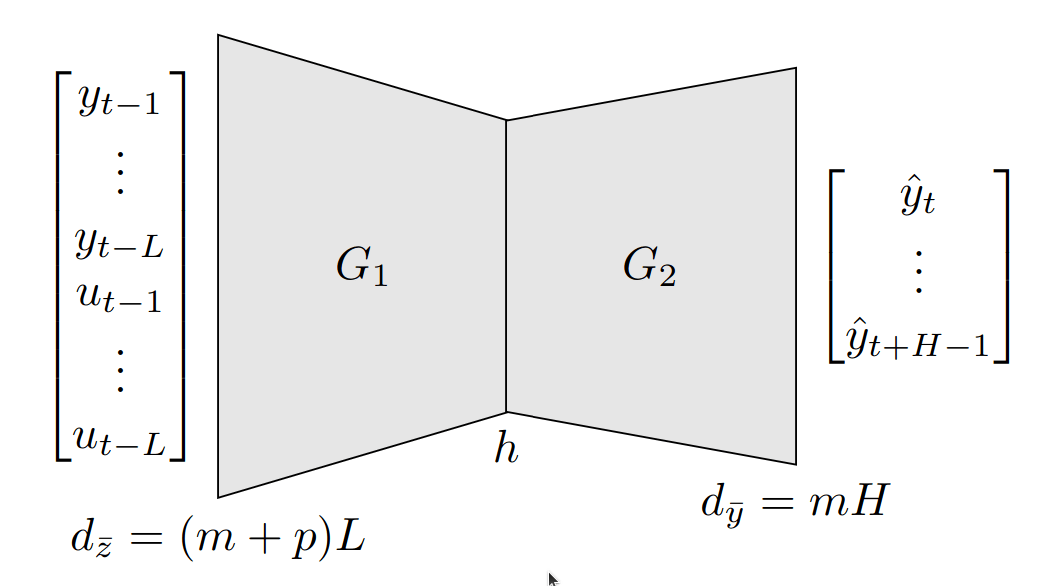
two layer linear network

Question: will model activations recover the Kalman filter state estimate, up to similarity transform?

squared loss $ \displaystyle \min \frac{1}{2T} \sum_{t=1}^T \Vert{}y_{t:t+H-1} - G_2 G_1 {z}_t\Vert{}_{2}^2$

$z_t:=$

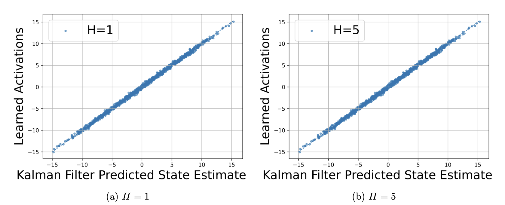
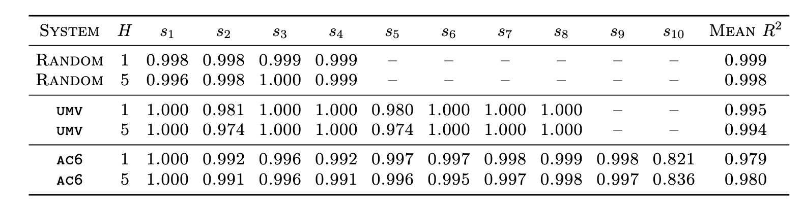
Main result

SS-KF on $\{u_k, y_k\}_{k=0}^{t-1}$

Assumptions: Linear-Gaussian system with

Non-explosive, i.e. $\rho(A) = \max |\lambda_i(A)| \leq 1$
Observable, i.e. $\begin{bmatrix}C^\top & (CA)^\top & \dots &(CA^{d_x-1})^\top\end{bmatrix}^\top$ is full rank
Persistent excitation, $\Sigma_w, \Sigma_v\succ 0$ and training $\{u_t\}_{t=0}^{T-1} \sim \mathcal N(0,I)$

similarity transform

model dimension

Proposition (Informal). The optimization landscape is benign.

Yahya Sattar

ICML '26

Theorem (Informal). Let $d_h=d_x$ and $H \geq d_x$ and $L \gtrsim \log(T) / (1 - \rho_\mathrm{KF})$.

Fix $\delta,\epsilon>0$. Assume $T \gtrsim \max\left\{ L \left(d_{z} + \log\left(\frac{T}{\delta}\right)\right), \frac{BH}{\epsilon} \left(d_x (H d_{y} + d_{z}) + \log \left(\frac{T}{\delta}\right)\right) \right\}.$
Then, for any $B$-bounded $\{u_k, y_k\}_{k=0}^{t-1}$, with probability at least $1 - \delta$ , $$\min_{S\in\text{GL}_{d_x}(\mathbb R)}\Vert{}Sh_t-\hat{x}_{t|t-1}\Vert{}_{2}^2 \lesssim \epsilon$$

filter stability

Proof outline

$\|S h_t - \hat x_t \|^2 = \|S \hat G_1 z_t - G^\star_1 z_t + G^\star_1 z_t - \hat x_{t|t-1} \|^2$

$ \leq 2\|S \hat G_1 - G_1^\star \|^2\|z_t\|^2 +2\|G^\star_1 z_t - \hat x_{t|t-1} \|^2$
$\leq \frac{10\|z_t\|^2}{\sigma_{\min}(G_2^\star G_2^\star{}^\top, G_1^\star G_1^\star{}^\top)}\| \hat G_2 \hat G_1 - G_2^\star G_1^\star\|^2\ + 2\|G^\star_1 z_t - \hat x_{t|t-1} \|^2$
Lemma: Procrustes distance bound holds if $\| \hat G_2 \hat G_1 - G_2^\star G_1^\star\|^2$ small

Recall that for the steady state Kalman filter, $$\hat x_{t+1|t} = \underbrace{(A-ALC)}_{\bar A} \hat x_{t|t-1} + B u_{t} + \underbrace{AL}_{F} y_{t} ,\qquad y_t = C \hat x_{t|t-1} + C(x_t-\hat x_{t|t-1}) + v_t$$
As a consequence, $$\hat{x}_{t|t-1} = \underbrace{\begin{bmatrix}F & \dots & \bar{A}^{L-1}F & B & \dots & \bar{A}^{L-1}B \end{bmatrix}}_{G_1^\star} {z}_t + \bar{A}^L \hat{x}_{t-L},\qquad y_{t:t+H-1} =\underbrace{ \begin{bmatrix} C \\ CA \\ \vdots \\ CA^{H-1} \end{bmatrix}}_{G_2^\star }\hat{x}_{t|t-1} + \xi_t $$

Proof outline

$$\hat{x}_{t|t-1} = {G_1^\star} {z}_t + \bar{A}^L \hat{x}_{t-L},\qquad y_{t:t+H-1} ={G_2^\star }\hat{x}_{t|t-1} + \xi_t $$

$\|S h_t - \hat x_t \|^2 = \|S \hat G_1 z_t - G^\star_1 z_t + G^\star_1 z_t - \hat x_{t|t-1} \|^2$

$ \leq 2\|S \hat G_1 - G_1^\star \|^2\|z_t\|^2 +2\| \bar{A}^L \hat{x}_{t-L} \|^2$
$\leq \frac{10\|z_t\|^2}{\sigma_{\min}(G_2^\star G_2^\star{}^\top, G_1^\star G_1^\star{}^\top)}\| \hat G_2 \hat G_1 - G_2^\star G_1^\star\|^2\ + 2\| \bar{A}^L \hat{x}_{t-L}\|^2$
Lemma: Procrustes distance bound holds if $\| \hat G_2 \hat G_1 - G_2^\star G_1^\star\|^2$ small
$\leq\frac{ 10 \|z_t\|^2}{\sigma_{\min}(G_2^\star G_2^\star{}^\top, G_1^\star G_1^\star{}^\top)}\frac{1}{\lambda_{\min}(\sum_{t=1}^T z_tz_t^\top)} \sum_{t=1}^T \| (\hat G_2 \hat G_1 - G_2^\star G_1^\star)z_t\|^2 + 2\| \bar{A}^L \hat{x}_{t-L} \|^2$

properties of optimal KF

truncation error, decays geometrically in $L$

Theorem: in-sample prediction error $$\lesssim H\left(d_x (H d_{{y}} + d_{{z}}) + \log \left(\frac{T}{\delta}\right)\right)$$

Theorem: persistent excitation $$\sum_{t=1}^T z_t z_t^\top \succsim T I$$

Proof outline

$$\hat{x}_{t|t-1} = {G_1^\star} {z}_t + \bar{A}^L \hat{x}_{t-L},\qquad y_{t:t+H-1} ={G_2^\star }\hat{x}_{t|t-1} + \xi_t $$

$\|S h_t - \hat x_t \|^2 = \|S \hat G_1 z_t - G^\star_1 z_t + G^\star_1 z_t - \hat x_{t|t-1} \|^2$

$ \leq 2\|S \hat G_1 - G_1^\star \|^2\|z_t\|^2 +2\| \bar{A}^L \hat{x}_{t-L} \|^2$
$\leq \frac{10\|z_t\|^2}{\sigma_{\min}(G_2^\star G_2^\star{}^\top, G_1^\star G_1^\star{}^\top)}\| \hat G_2 \hat G_1 - G_2^\star G_1^\star\|^2\ + 2\| \bar{A}^L \hat{x}_{t-L}\|^2$
$\leq\frac{ 10 \|z_t\|^2}{\sigma_{\min}(G_2^\star G_2^\star{}^\top, G_1^\star G_1^\star{}^\top)}\frac{1}{\lambda_{\min}(\sum_{t=1}^T z_tz_t^\top)} \sum_{t=1}^T \| (\hat G_2 \hat G_1 - G_2^\star G_1^\star)z_t\|^2 + 2\| \bar{A}^L \hat{x}_{t-L} \|^2$
$\lesssim \frac{H}{T} \left(d_x (H d_{{y}} + d_{{z}}) + \log \left(\frac{T}{\delta}\right)\right) \Vert{}{z}_t\Vert{}_{2}^2 $ as long as $$L \gtrsim \log(T) / (1 - \rho),\qquad T \gtrsim L \left(d_{{z}} + \log(T/\delta)\right)\:.$$

Main result

Theorem (Informal). Let $d_h=d_x$ and $H \geq d_x$ and $L \gtrsim \log(T) / (1 - \rho_\mathrm{KF})$.

Fix $\delta,\epsilon>0$. Assume $T \gtrsim \max\left\{ L \left(d_{z} + \log\left(\frac{T}{\delta}\right)\right), \frac{BH}{\epsilon} \left(d_x (H d_{y} + d_{z}) + \log \left(\frac{T}{\delta}\right)\right) \right\}.$
Then, for any $B$ bounded $\{u_k, y_k\}_{k=0}^{t-1}$, with probability at least $1 - \delta$ ,

$$\min_{S\in\text{GL}_{d_x}(\mathbb R)}\Vert{}Sh_t-\hat{x}_{t|t-1}\Vert{}_{2}^2 \lesssim \epsilon$$

1. Sequences have low rank auto-regressive structure

$y_{t:t+H-1} \approx G_2^\star G_1^\star {z}_t$

2. Small prediction errors imply small parameter errors (excitation)

$\hat G_2\hat G_1 z_t \approx G_2^\star G_1^\star z_t $ for all $t$

$\implies$

$\hat G_2\hat G_1 \approx G_2^\star G_1^\star $

Three ingredients:

$z_t$

$$\min \frac{1}{2T} \sum_{t=1}^T \Vert{}y_{t:t+H-1} - G_2 G_1 {z}_t\Vert{}_{2}^2$$

3. Small end-to-end errors imply small first layer errors

$\hat G_2\hat G_1 \approx G_2^\star G_1^\star $

$\implies$

$S\hat G_1 \approx G_1^\star $

Opportunity for new provable learning and control algorithms based on (deep) end-to-end training
- KF mean $\hat x_t$ is sufficient for optimal quadratic control
Hidden state (posterior) recovery is limited by data
- cannot recover latent quantities absent from data, whether due to lack of observability or excitation
Open question: expand theory beyond linear-Gaussian?
- Key challenge: tractability of optimal filter (nonlinear)
- Idea: study best filter within function class, e.g. class of linear filters
Open question: what part of posterior do we expect to recover in general? ($\hat x_t$ vs. $\Sigma_t$?)

Implications and open questions

Outline:

1. Recovering Latent States

2. Control from Partial Observation

filter

controller

$y$

$u$

system

$x$

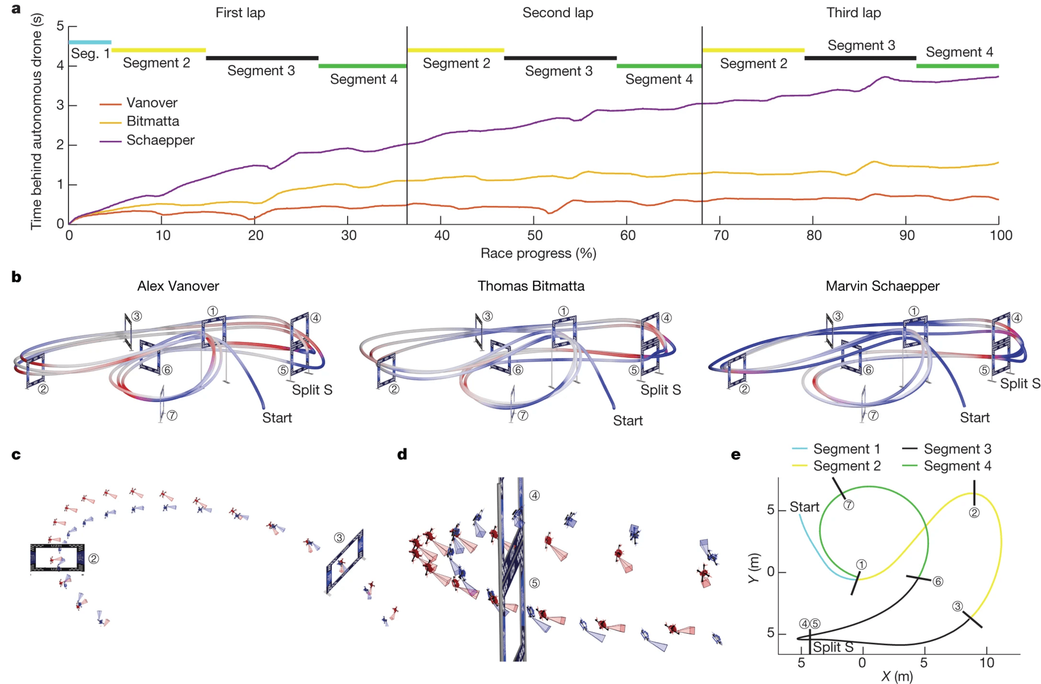
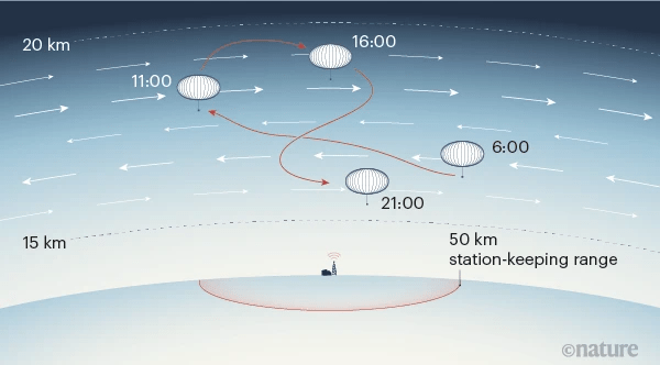
Observer effects occur when there is coupling between actuation and observation

examples: electronic circuits, quantum wave collapse, human psychology, robotics ....

Observer Effects

Linear state update with $A\in\mathbb R^{n\times n}$, $B\in\mathbb R^{n\times p}$ $$x_{t+1} = Ax_t + Bu_t + w_t $$
Bilinear measurements with $C_i\in\mathbb R^{m\times n}$ $$y_t = \underbrace{\Big(C_0 + \sum_{i=1}^p u_t[i] C_i \Big)}_{C(u_t)}x_t + v_t$$
Gaussian process noise, measurement noise, and initial state $$\{w_t\} \sim \mathcal N(0,\Sigma_w),\quad \{v_t\} \sim \mathcal N(0, \Sigma_v),\quad x_0 \sim \mathcal N(0,\Sigma_0)$$

Bilinear Observation

Belief state via the Kalman Filter: $x_t|\mathcal I_t \sim \mathcal N(\hat x_t,\Sigma_t)$

$\hat x_{t+1} = A\hat x_t + Bu_t - L_t\big(y_t-C(u_t)\hat x_t\big)$

$\Sigma_{t+1} = (A+ L_tC(u_t))\Sigma_tA^\top + \Sigma_w$

$L_t = -A\Sigma_tC(u_t)^\top(C(u_t)\Sigma_tC(u_t)^\top+\Sigma_v)^{-1}$

Problem Setting: Optimal Control

$$\min_{u_t=\pi_t(\mathcal I_t)} \mathbb E\left[x_T^\top Q x_T+ \sum_{t=1}^{T-1} x_t^\top Q x_t + u_t^\top R u_t \right]\\ \text{s.t.} \quad x_{t+1} = Ax_t + Bu_t + w_t \\\qquad\qquad\qquad y_t =\Big(C_0 + \sum_{i=1}^p u_t[i] C_i \Big)x_t + v_t$$

Small departure from classic LQG control

Sunmook Choi

Yahya Sattar

Yassir Jedra

Maryam Fazel

Leo Maynard-Zhang

$$\mathcal I_t = \{u_0,...,u_{t-1}, y_0, ..., y_{t-1}\}$$ information set for decision-making

quadratic costs ($Q,R\succ 0$)

"Certainty Equivalent" Separation Principle

Separation principle (SP): independently design
estimation & control
- Optimal for partially observed
  LQ control ($C_i=0$ for $i>0$)
The SP policy has two components:
1. State estimation $\hat x_t = \mathbb E[x_t|\mathcal I_t]$ (Kalman filter)
2. State dependent policy $u_t = K^\star_t \hat x_t$ (LQR $K^\star$)

Kalman

Filter

State Feedback

$y$

$\hat x$

$u$

Pitfalls of Separation

Theorem: For $T\geq 2$, the optimal policy is not affine in the estimated state.
- As a consequence, the SP policy is not optimal
In addition, we construct examples where
- The SP policy locally maximizes the cost
- The SP policy is essentially an open-loop policy

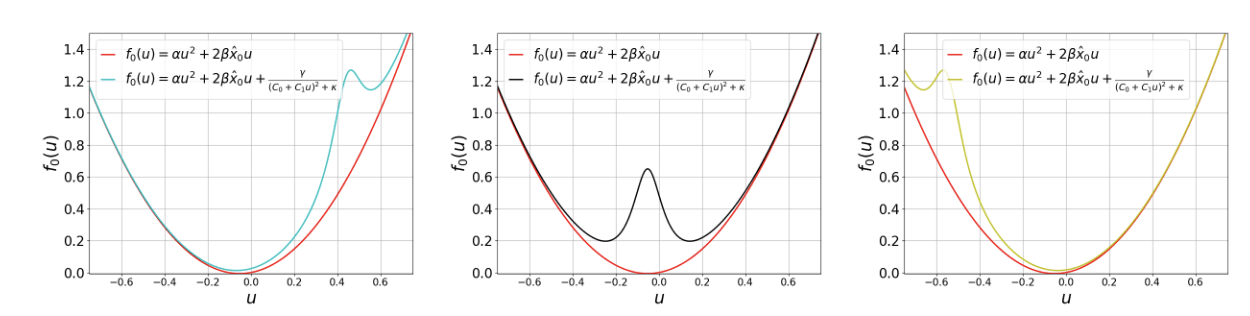
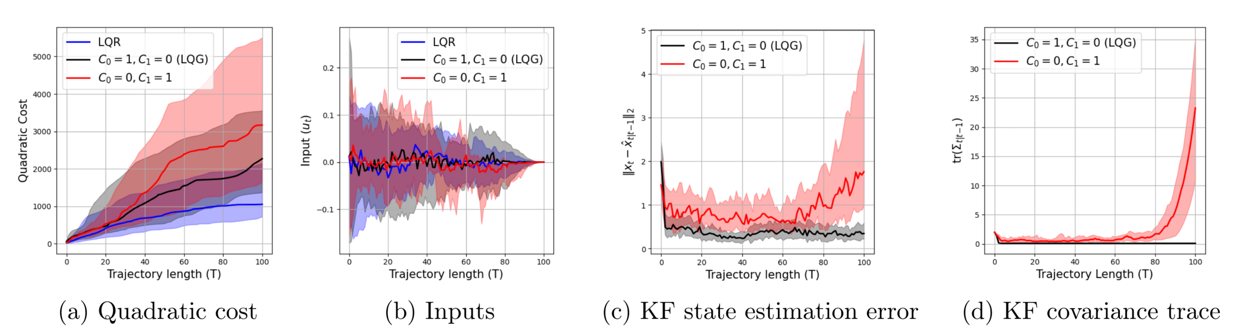
Examples where SP is bad

$$\begin{align*} x_{t+1} &= \begin{bmatrix} 1 & 0.3 \\ 0 & 1\end{bmatrix} x_t + \begin{bmatrix}0.3 \\ 0 \end{bmatrix} u_t + w_t \\ y_t &= u_t\begin{bmatrix} 1 & 0\end{bmatrix} x_t + v_t \end{align*}$$

with $Q=I$ and $R=1000$

$$\begin{align*} x_{t+1} &= x_t + \begin{bmatrix}0 & 1 \end{bmatrix} u_t + w_t \\ y_t &= u_t^\top \begin{bmatrix} 1\\ 0\end{bmatrix} x_t + v_t \end{align*}$$

with $Q=\frac{1}{2}$ and $R=I$

$\implies$

infinite horizon $K_\star = \begin{bmatrix} 0 \\ \frac{1}{2}\end{bmatrix}$

$y_t = \hat x_t \begin{bmatrix} 0 \\ \frac{1}{2}\end{bmatrix}^\top \begin{bmatrix} 1 \\ 0\end{bmatrix} x_t + v_t$

$0$ only noise is observed!

Select a fixed "probing" action whenever all three hold:
1. no probing action has been taken recently
2. $|C(K_t^\star \hat x_t)|$ is small
3. $\bar\Sigma_{OL} - \Sigma_t$ is small
Otherwise, follow SP $K_t \hat x_{t}$
Theoretically and empirically improved performance

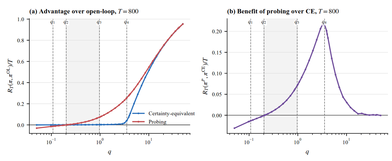
$\propto 1/\sigma_z^2$

Heuristic Policy

open loop steady-state covariance

Leo Maynard-Zhang

Approximately Optimal Control

Sunmook Choi

Yahya Sattar

$$\begin{align*}\min_{u_t=\pi_t(\hat x_t,\Sigma_t)}~~& \mathbb E\left[ \sum_{t=1}^{T-1} \hat x_t^\top Q \hat x_t + \mathrm{tr}(\Sigma_t) + u_t^\top R u_t \right]\\ \text{s.t.}~~& \hat x_{t+1} = A\hat x_t + Bu_t + L_t(C(u_t)\hat x_t - y_t)\\ &\Sigma_{t+1} = (A+ L_tC(u_t))\Sigma_tA^\top + \Sigma_w \end{align*}$$

$$\mathbb E\left[x_t^\top Q x_t \mid \mathcal I_t \right]= \hat x_t\top Q\hat x_t + \mathrm{tr}(Q\Sigma_t)$$

$$\begin{align*} \min_{u_t=\pi_t(\mathcal I_t)} ~~&\mathbb E\left[\sum_{t=1}^{T-1} x_t^\top Q x_t + u_t^\top R u_t \right]\\ \text{s.t.}~~& x_{t+1} = Ax_t + Bu_t + w_t \\& y_t =C(u_t)x_t + v_t\end{align*}$$

$L_t = -A\Sigma_tC(u_t)^\top(C(u_t)\Sigma_tC(u_t)^\top+\Sigma_v)^{-1}$

Andrew Lowitt

Beixi Du

Daniel Cao

Rewrite OCP in terms of the belief space from KF

This is now a fully observed, nonlinear, stochastic optimal control problem

innovations $\sim \mathcal N(0, C(u_t)\Sigma_t C(u_t)^\top + \Sigma_v)$

Approximately Optimal Control

$$\begin{align*}\pi(\hat x_t,\Sigma_t)=\arg \min_{u_k}~~& \mathbb E\left[ \sum_{k=1}^{H} \bar x_k^\top Q \bar x_k + \mathrm{tr}(\bar\Sigma_k) + u_k^\top R u_k \right]\\ \text{s.t.}~~& \bar x_{k+1} = A\bar x_k + Bu_k\\ &\bar\Sigma_{k+1} = (A+ L_kC(u_k))\Sigma_kA^\top + \Sigma_w \\ &\bar x_0 = \hat x_t ,~~ \bar \Sigma_0=\Sigma_t\end{align*}$$

$L_t = -A\Sigma_tC(u_t)^\top(C(u_t)\Sigma_tC(u_t)^\top+\Sigma_v)^{-1}$

Rewrite OCP in terms of the belief space from KF

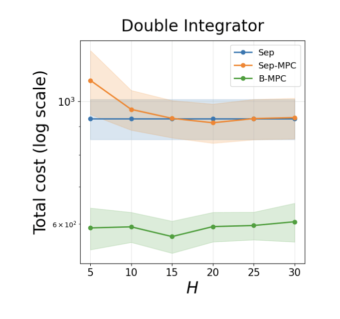
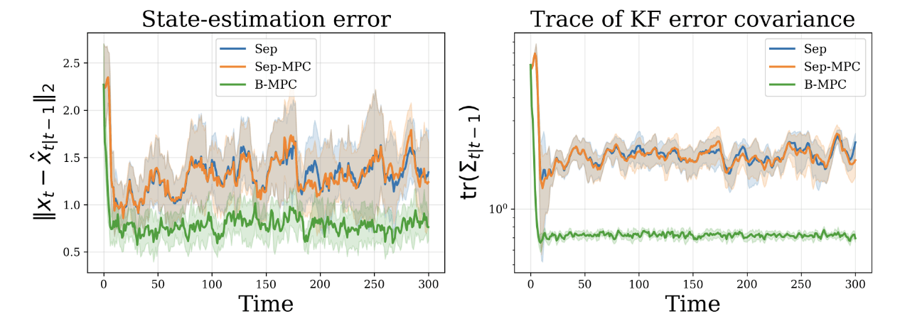
Expected dynamics, open loop inputs, finite horizon $\rightarrow$ MPC

"Solve" MPC problem with autograd and L-BFGS

Foundations of a simple model for studying partially observed control
Open question: do "world models" learn belief states, or only the mean/MLE?
- For purely linear dynamics, uncertainty (e.g. $\Sigma_t$) is not naturally in hidden activations
Open question: do reinforcement learning algorithms automatically recover uncertainty-aware behavior?
- e.g. caution under uncertainty, probing to gather information

Implications and open questions

Two-Layer Linear Auto-Regressive Models Estimate Latent States at ICML26 (arxiv:2606.12691) with Yahya Sattar, Sunmook Choi, Leo Maynard-Zhang, Yassir Jedra, Maryam Fazel
Sub-optimality of the Separation Principle for Quadratic Control from Bilinear Observations at CDC25 (arxiv:2504.11555) with Yahya Sattar, Sunmook Choi, Yassir Jedra, Maryam Fazel
Dual Control of Linear Systems from Bilinear Observations with Belief Space Model Predictive Control (arXiv:2604.24663) with Daniel Cao, Beixi Du, Andrew Lowitt, Sunmook Choi, Yahya Sattar
Performance Gaps Between Open-Loop, Certainty-Equivalent, and
Optimal Control Under Action-Dependent Observations with Leo Maynard-Zhang, Sunmook Choi, Yahya Sattar, Yassir Jedra, Maryam Fazel

Thanks! Questions?

Sunmook Choi

Yahya Sattar

Yassir Jedra

Maryam Fazel

Leo Maynard-Zhang

Andrew Lowitt

Beixi Du

Daniel Cao

Setting: generate sequence with arbitrary Hidden Markov Model $(A,B)$. Provide LLM with sequence only $$(o_1,o_2,...,o_t)$$
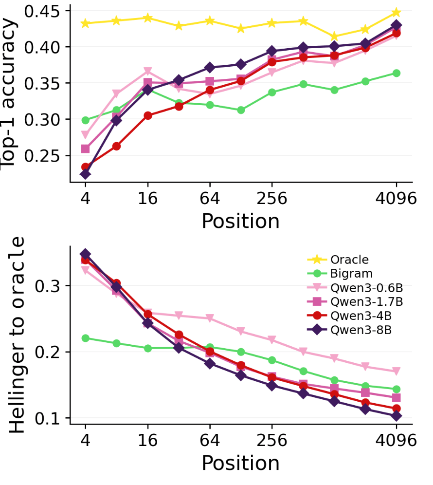
Observation: as LLMs observe longer sequences, their predictions converge towards that of the true posterior

"Real" Models, Synthetic Data

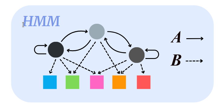
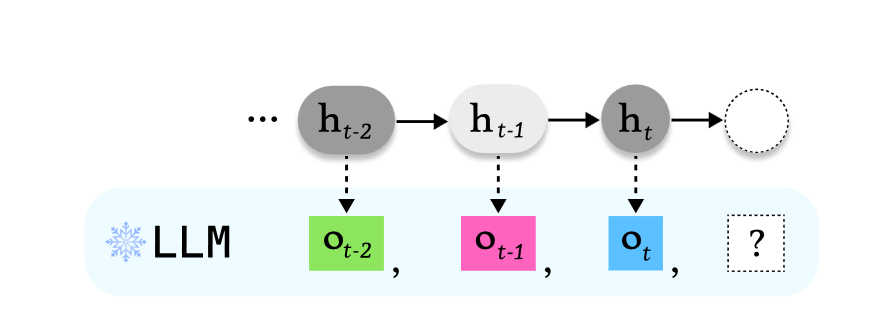
Yijia Dai

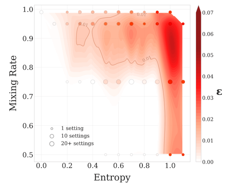
Dai et al., Pre-trained Large Language Models Learn Hidden Markov Models In-context

Setting: generate sequences with fixed stochastic Linear Dynamical System $(A,B,C,\Sigma_w,\Sigma_v)$.
Train two-layer linear network
Observation: for sufficiently large training data, the hidden activations align with the Kalman filter state estimate

Simple Models, Synthetic Data

Sattar et al., Two-Layer Linear Auto-Regressive Models Estimate Latent States

$x$

$A, B$

$C$

$w$

$v$

$u$

$y$

Sunmook Choi

Leo Maynard-Zhang