CS 4/5789: Introduction to Reinforcement Learning

Lecture 25: AlphaGo Case Study

Prof. Sarah Dean

MW 2:55-4:10pm
255 Olin Hall

Reminders

• Homework
  • 5789 Paper Assignments
  • Prelim corrections due by Final
• Final exam is Tuesday 5/14 at 2pm in Ives 305
  • Will post review slides, PSet solutions, and draft notes on MAB/Exploration

Agenda

1. Recap: Units 1-3

2. Game Setting

3. Policy Learning Component

4. Value Learning Component

5. Online Planning Component

• Unit 1:
  • Optimal Policies in MDPs: VI, PI, DP, LQR
• Unit 2:
  • Learning Value/Q, Policies
• Unit 3:
  • Exploration & bandits
  • Expert demonstration

Recap:

1: MDPs & Optimal Policies

• Tabular MDPs: VI, PI, and DP
• Continuous Control: LQR via DP

action \(a_t\)

state \(s_t\)

reward \(r_t\)

policy \(\pi\)

transitions \(P,f\)

2: Policies from Data

• Learning Value/Q Functions
• Optimizing Policies (by estimating gradients)

action \(a_t\)

state \(s_t\)

reward \(r_t\)

policy

data \((s_t,a_t,r_t)\)

policy \(\pi\)

transitions \(P,f\)

experience

unknown

3A: Bandits & Exploration

• Multi-Armed/Contextual Bandits
• Upper Confidence Bound Algorithms

3B: Learning from Expert

Supervised Learning

Policy

\((x=s, y=a^*)\)

Goal: understand/predict behaviors

Agenda

1. Recap: Units 1-3

2. Game Setting

3. Policy Learning Component

4. Value Learning Component

5. Online Planning Component

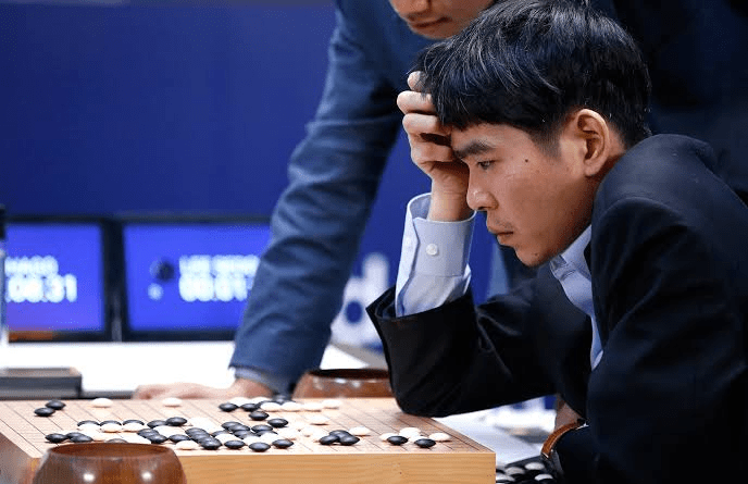
AlphaGo vs. Lee Sedol

49:30-56:30

...

Setting: Markov Game

• Two Player Markov Game: \(\{\mathcal S,\mathcal A, f, r, H, s_0\}\)
• Deterministic transitions: \(s' = f(s,a)\)
• Players alternate taking actions:
  • Player 0 in even steps, player 1 in odd steps
• Sparse reward: \(r(s_H)=1\) when player 0 wins (else \(-1\))

Mastering the game of Go with deep neural networks and tree search, 2016

...

Setting: Markov Game

• Min-max formulation $$ V^*(s) =  \textcolor{red}{\max_{\pi_0} } \textcolor{yellow}{\min_{\pi_1} }\mathbb E[r(s_H)|s_0=s, \pi_1, \pi_2]$$
• Zero sum game

Setting: Markov Game

• Min-max formulation $$ V^*(s) =  \textcolor{red}{\max_{\pi_0} } \textcolor{yellow}{\min_{\pi_1} }\mathbb E[r(s_H)|s_0=s, \pi_1, \pi_2]$$
• Zero sum game \(\implies\) solvable with DP!

Setting: Markov Game

• But \(H\approx 150\), \(A\approx 250\), so this tree will have \(\approx A^H\) nodes
• 1 TB hard-drive can store \(\approx 250^6\) 8-bit numbers
• Impossible to enumerate!

\(V^*(s) = \max\{Q^*(s,a), Q^*(s,a')\}\)

\(Q^*(s,a) = V^*(f(s,a))\)

\(V^*(s') = \min\{Q^*(s',a), Q^*(s',a')\}\)

Setting: Markov Game

Strategy:

• Approximate \(\pi^*\), use \(\widehat \pi\) to approximate \(V^*\) as \(\widehat V\)
• Low depth tree search combines \(\widehat V\) with simulated play \(\widehat \pi\)

\(V^*(s) = \max\{Q^*(s,a), Q^*(s,a')\}\)

\(Q^*(s,a) = V^*(f(s,a))\)

\(V^*(s') = \min\{Q^*(s',a), Q^*(s',a')\}\)

Agenda

1. Recap: Units 1-3

2. Game Setting

3. Policy Learning Component

4. Value Learning Component

5. Online Planning Component

Policy Learning

Deep network with convolutional layers

• input: 19x19 3-bit grid
• output: distribution over grid

Imitation Learning

Warm-start policy network with expert data

1. Sample data \((s,a)\) from human games, \(N=30\) million
2. Log-likelihood loss function $$\min_\pi \sum_{i=1}^N -\log(\pi(a_i|s_i))$$
3. Optimize with Stochastic Gradient Descent $$ \theta_{t+1} = \theta_t - \eta \frac{1}{|\mathcal B|} \sum_{(s,a)\in \mathcal B}-\nabla_\theta\log(\pi_\theta(a|s))$$

Imitation Learning

How well does \(\pi_{\theta_{BC}}\) perform?

• 57% accuracy on held out test
  • random policy: 1/200
• Pachi: open source Go program
  • 11% win rate

Policy Gradient

1. Warm-start \(\theta_0 = \theta_{BC}\)
2. Iterate for \(t=0,...,T-1\)
   1. Randomly select previous \(\tau \in \{0,1..., t\}\)
   2. Play \(\pi_{\theta_t}\) against \(\pi_{\theta_\tau}\) and observe \((s_0,\)\(a_0\)\(,s_1,\)\(a_1\)\(,...,s_H)\)
   3. Gradient update: $$\theta_{t+1} = \theta_t + \eta \sum_{h=0 }^{H/2}\nabla_\theta \log \pi_{\theta_t}(\textcolor{red}{a_{2h}}|s_{2h}) r(s_H)$$

Policy Gradient

How well does \(\widehat \pi = \pi_{\theta_{PG}}\) perform?

• Pachi: open source Go program
  • 85% win rate

Agenda

1. Recap: Units 1-3

2. Game Setting

3. Policy Learning Component

4. Value Learning Component

5. Online Planning Component

Value Learning

Deep network with convolutional layers

• input: 19x19 3-bit grid
• output: scalar value

Value Learning

• Ideally, approximate \(\widehat V \approx V^*\)
  • easier to supervise \(\widehat V \approx V^{\widehat \pi}\) $$V^{\widehat \pi}(s) = \mathbb E[s(r_H)|s_0=s, \widehat \pi, \widehat \pi]$$
• Supervision via rollouts
  • In each game \(i\), sample \(h\) and set \(s_i=s_h\) and \(y_i\) as the game's outcome (\(\pm 1\))
  • Simulate \(N=30\) million games

  • IID sampling \(s\sim d^{\widehat \pi}\)

Value Learning

• Least-squares regression $$\min_\beta \sum_{i=1}^N (V_\beta(s_i) - y_i)^2$$

• Optimize with SGD $$\beta_{t+1} = \beta_t - \eta \sum_{s,z\in\mathcal B} (V_{\beta}(s) - y) \nabla_\beta V_\beta(s)$$

Agenda

1. Recap: Units 1-3

2. Game Setting

3. Policy Learning Component

4. Value Learning Component

5. Online Planning Component

Combination with Search

Combination with Search

1. Low depth search: use knowledge of dynamics

\(a_t = \arg\max \widehat V(f(s_t,a))\)

Combination with Search

1. Low depth search: use knowledge of dynamics

Combination with Search

\(a_t = \)\(\arg\max_a\)\( \min_{a'} \)\(\max_{a''}\)\( \widehat V(f(f(f(s_t,a),a'),a''))\)

1. Low depth search: use knowledge of dynamics

Combination with Search

\(s'=f(s,a)\)

2. Improve value estimate with rollout

\(s''=f(s',a')\)

\(s'''=f(s'',a'')\)

Combination with Search

1. Low adaptive depth tree search with \(\widehat V\)
2. Improve value estimate with rollout of \(\widehat \pi\)

Summary

1. Learning:
   1. Warm start policy with imitation learning
   2. Improve policy with policy gradient
   3. Approximate value of policy
2. Planning:
   1. Adaptive tree search with \(\widehat V\) and \(\widehat \pi\)

AlphaGo vs. Lee Sedol

1:07-1:09

• AlphaGo Zero (2017)
  • Replaces imitation learning with random exploration
  • Uses MCTS during self-play
  • Single network for policy and value
• AlphaZero (2018)
  • Generalizes beyond Go to Chess and Shogi
  • Removes Go-specific design elements (e.g. symmetry)
• MuZero (2020)
  • Generalizes to Atari by not requiring dynamics \(f\)
  • Past observations \(o_{1:t}\) and hypothetical future actions \(a_{t:t+k}\) are inputs to a single policy/value network

To Alpha(Go) Zero and Mu Zero

"Real world" considerations