MexSIAM-2025

Yofre H. Garcia

Saúl Diaz-Infante Velasco

Jesús Adolfo Minjárez Sosa

sauldiazinfante@gmail.com

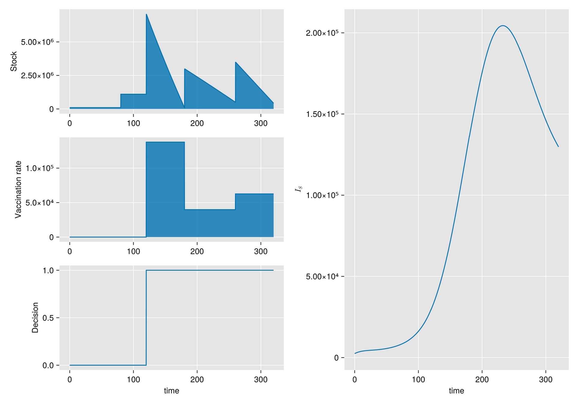
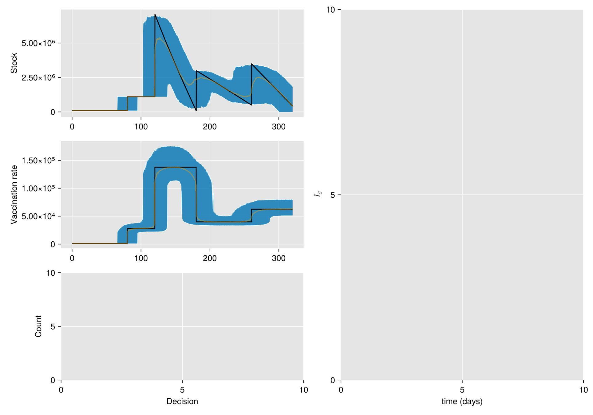
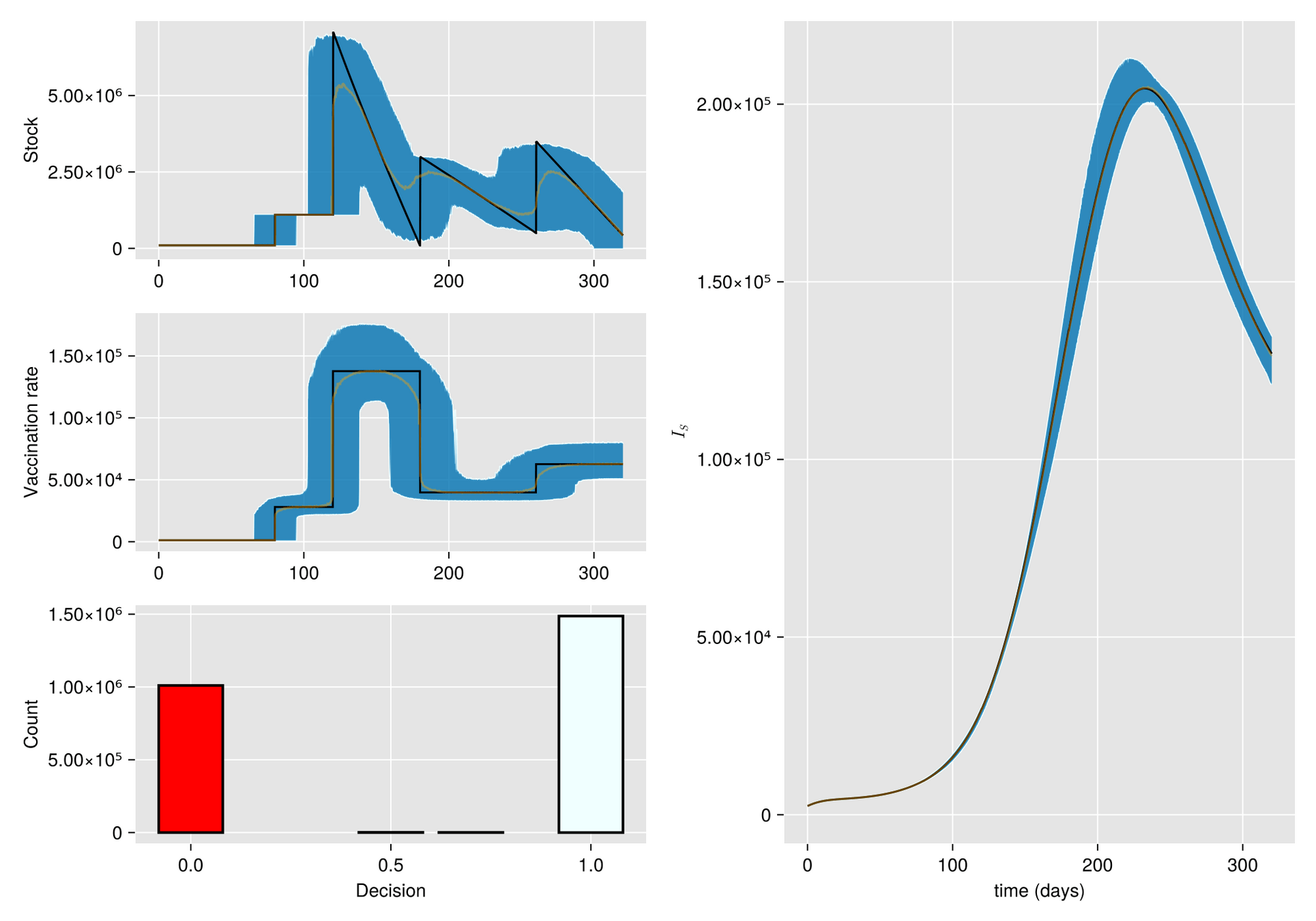
Argument. When there is a shortage of vaccines, sometimes the best response is to refrain from vaccination, at least for a while.

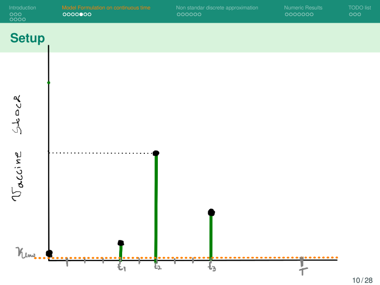
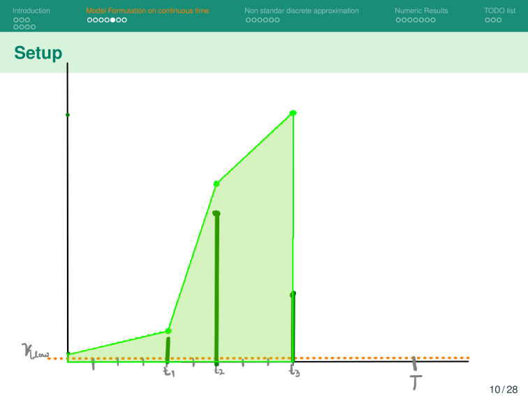
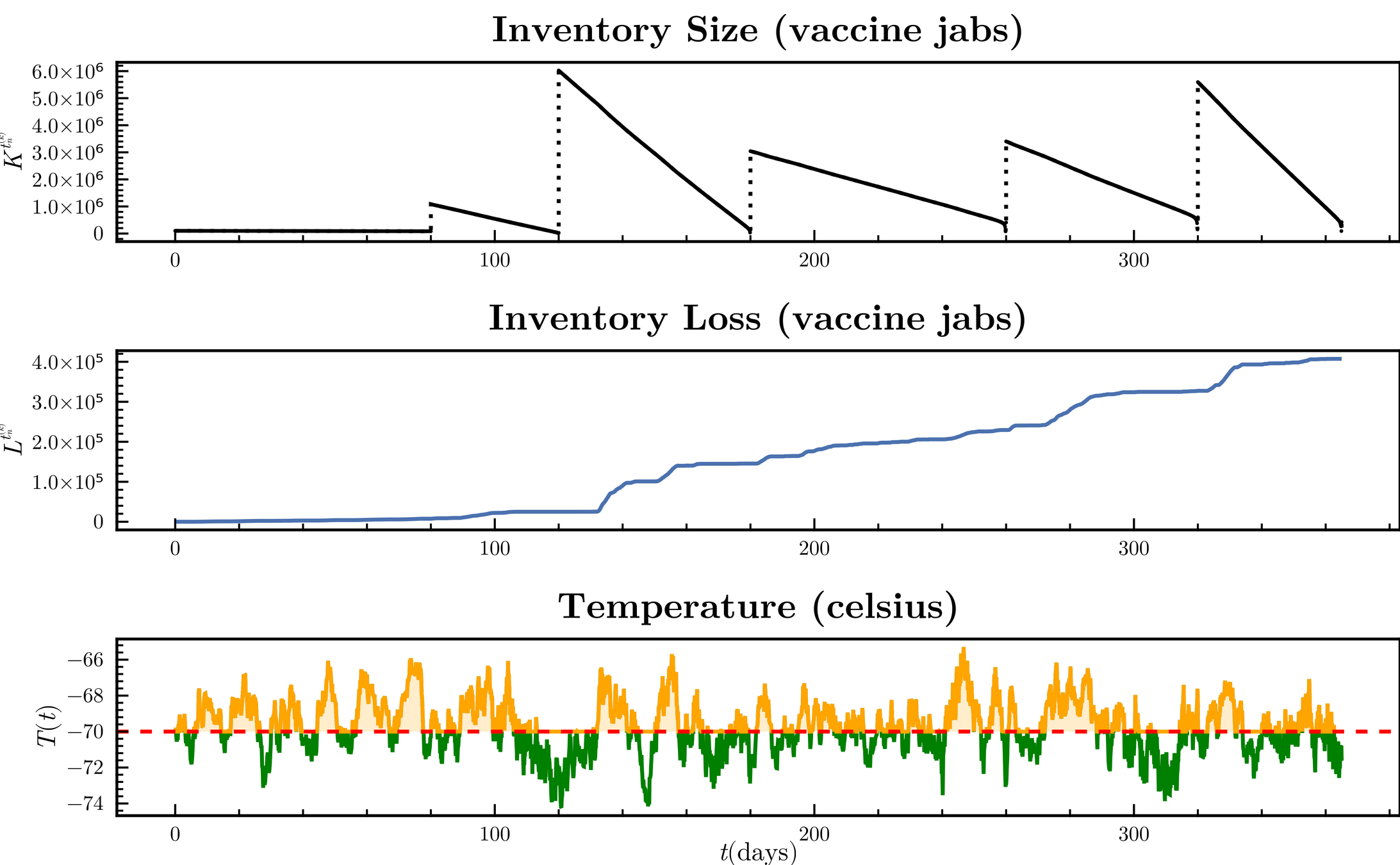
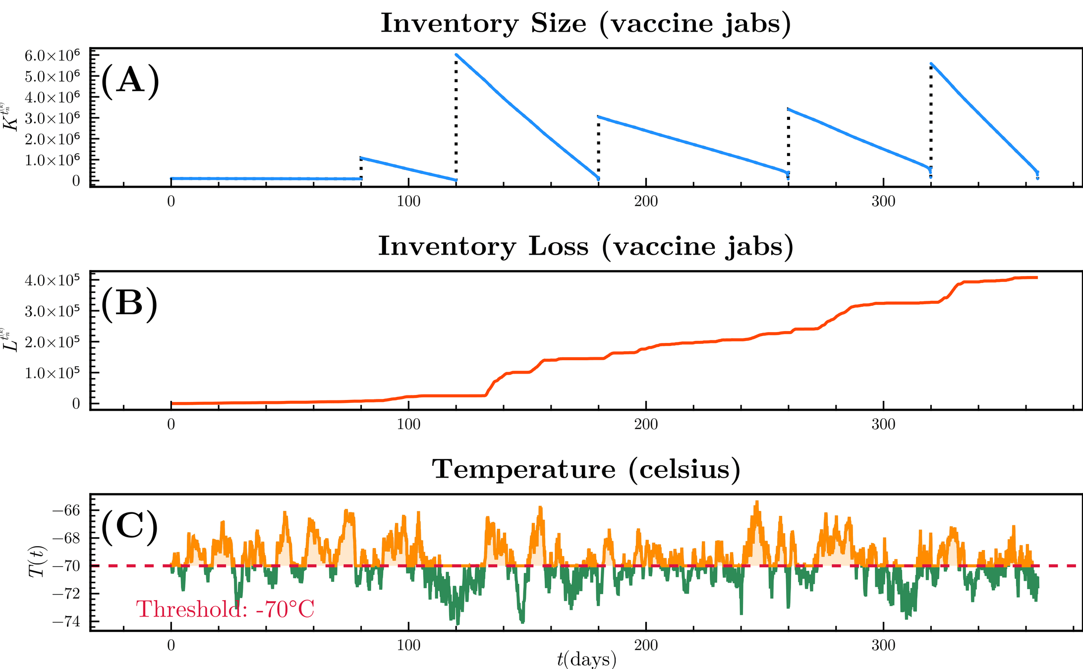
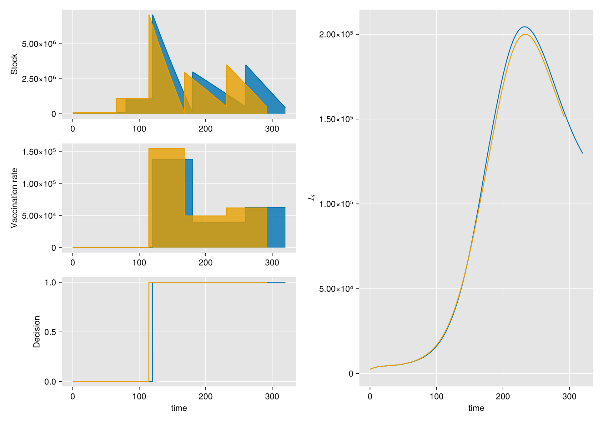
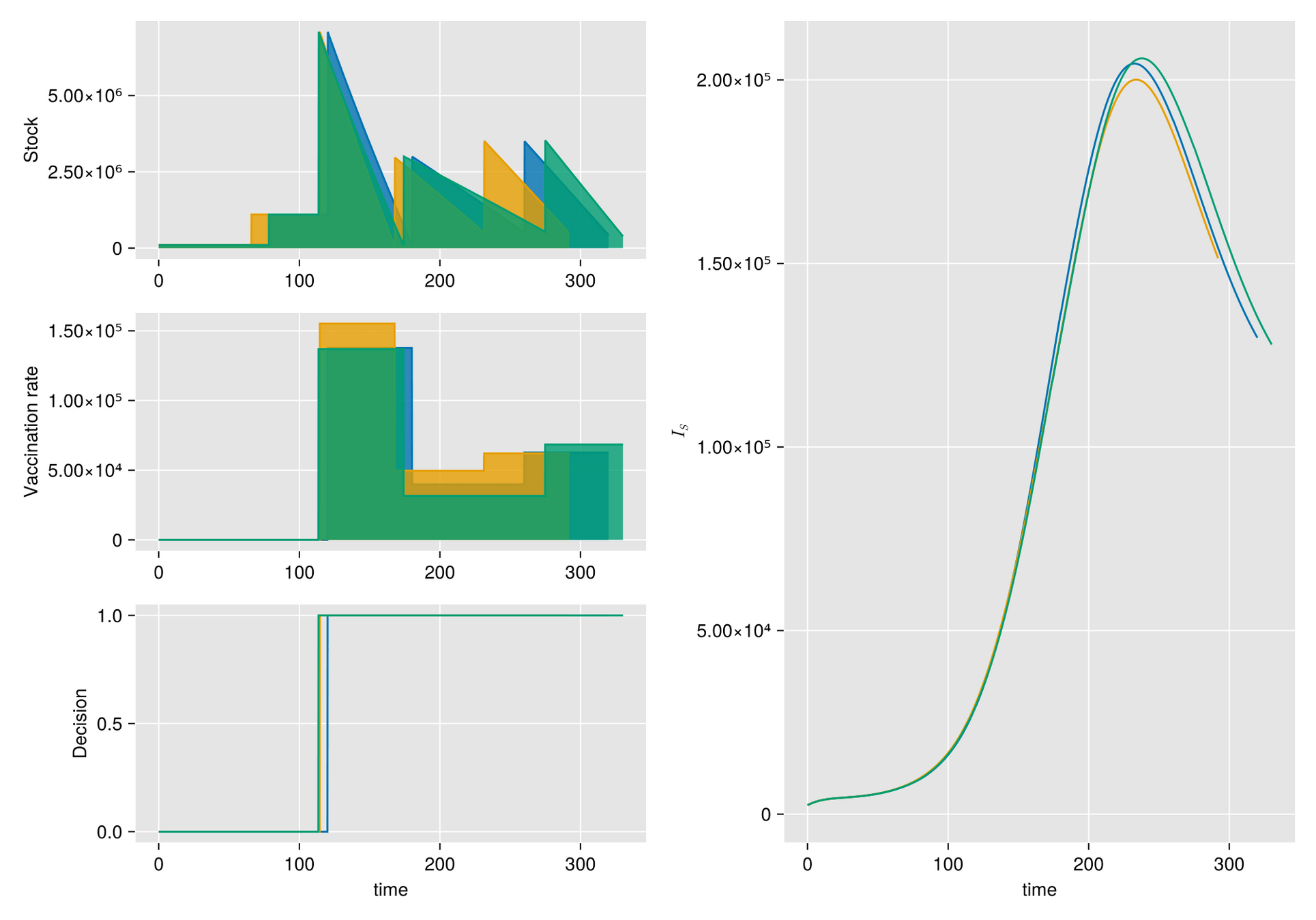
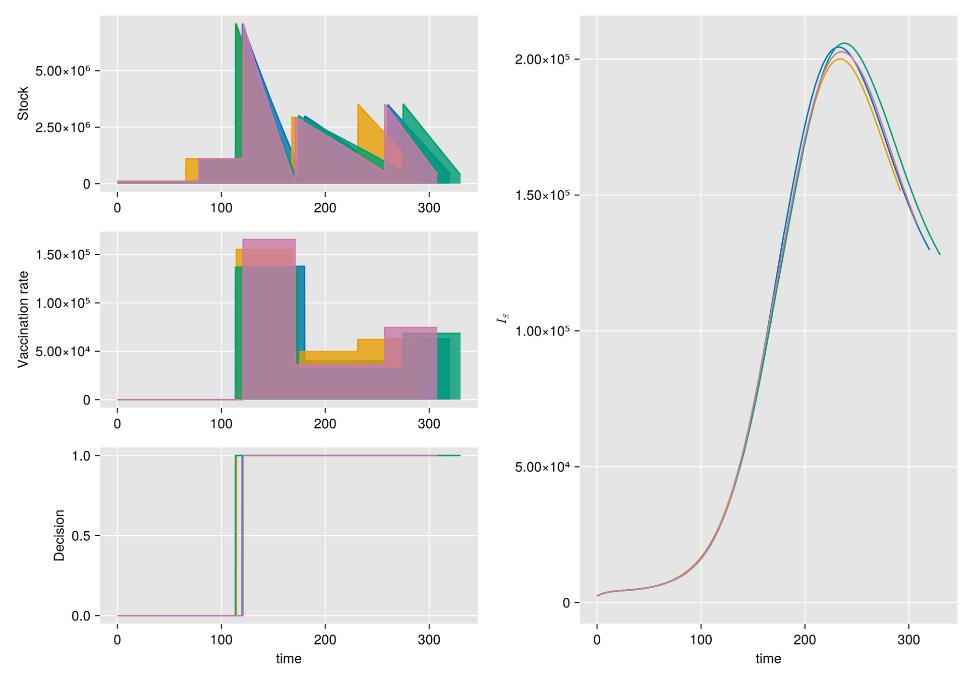
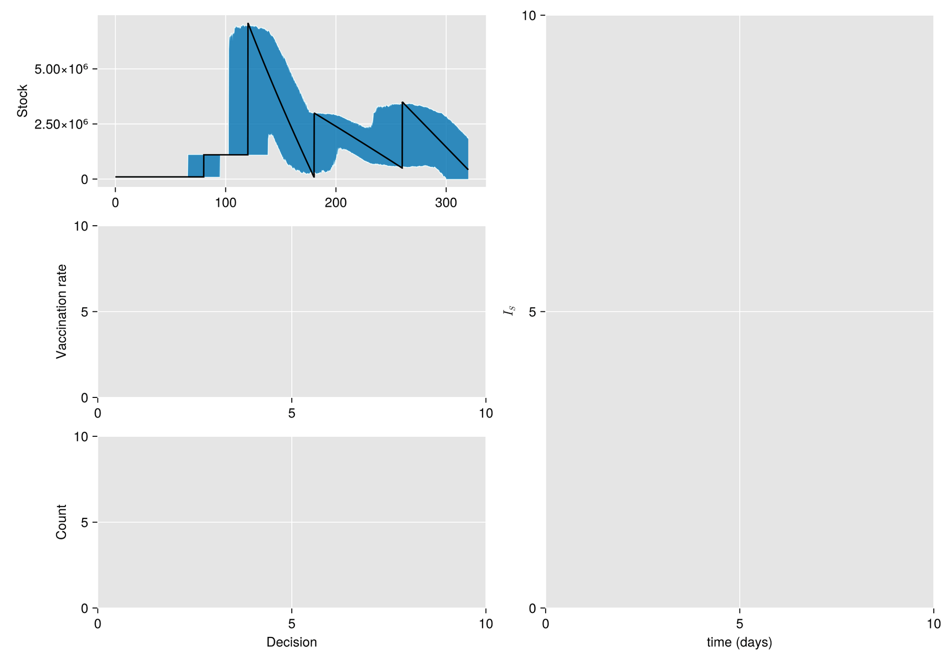
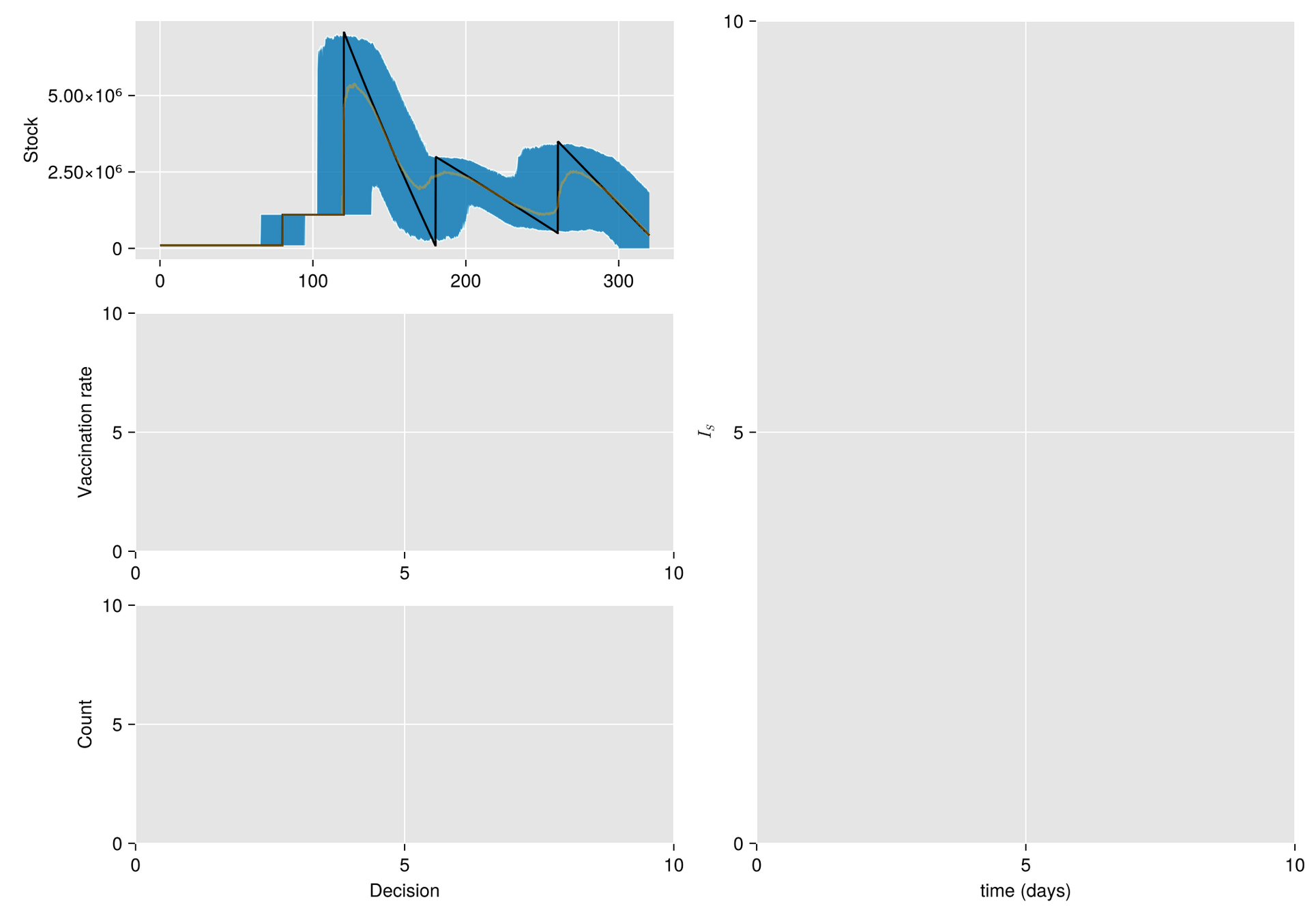
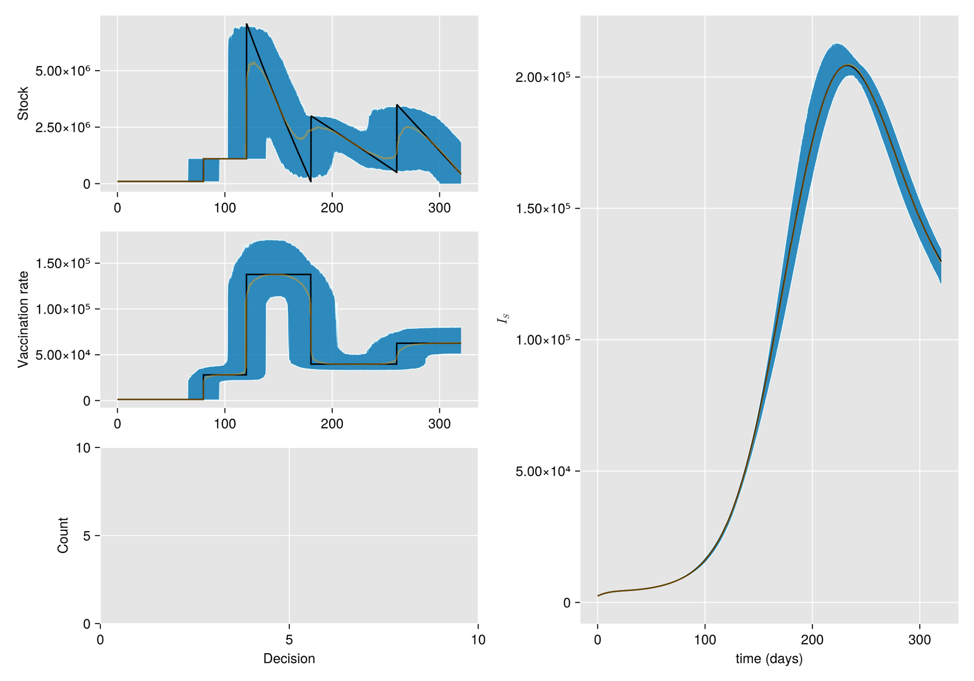
Hypothesis. Under these conditions, inventory management suffers significant random fluctuations

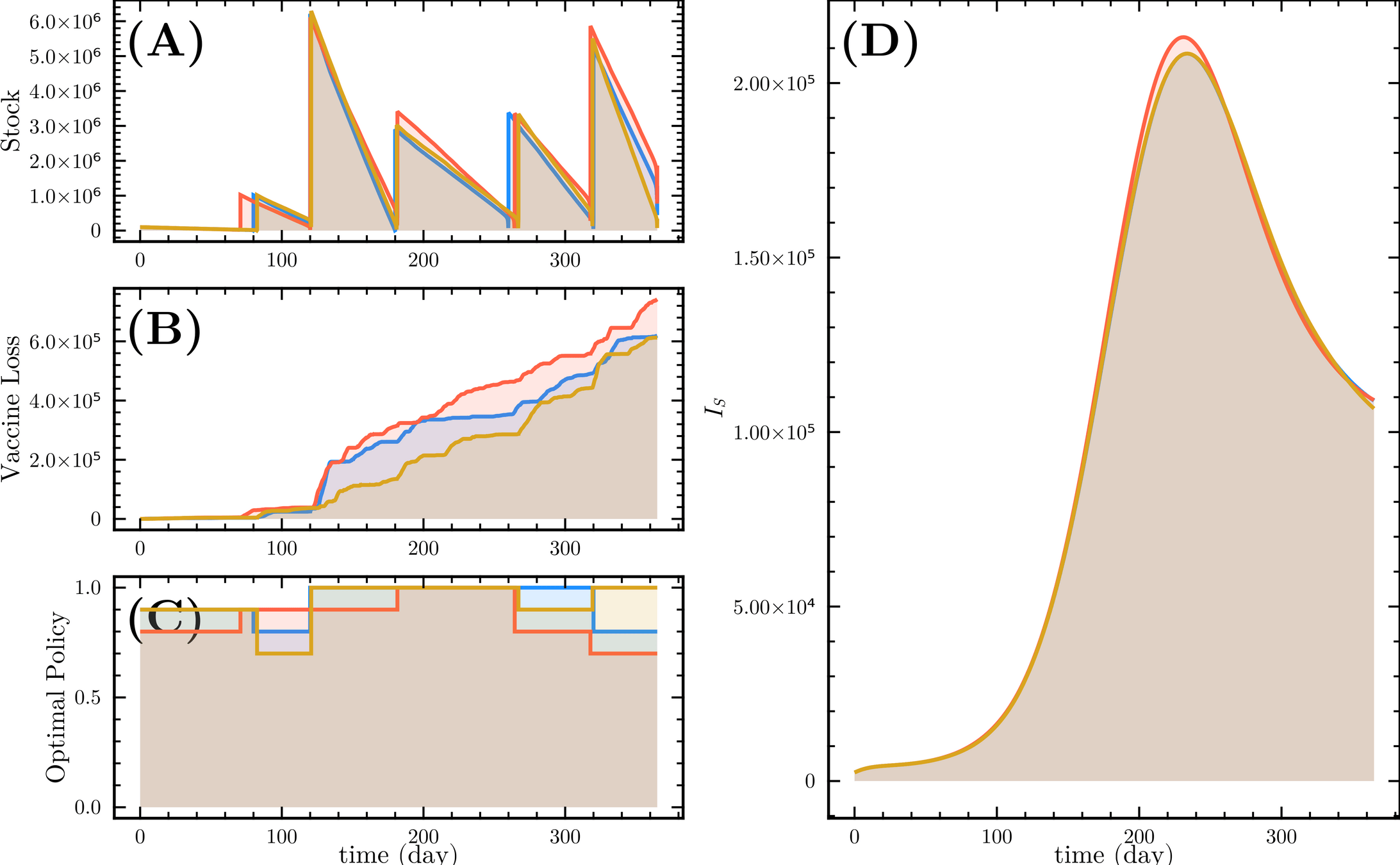
Objective. Optimize the management of vaccine inventory and its effect on a vaccination campaign

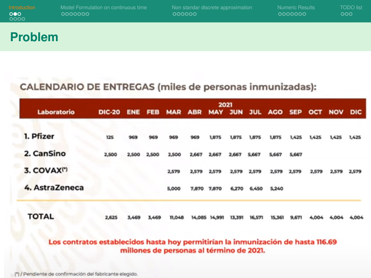
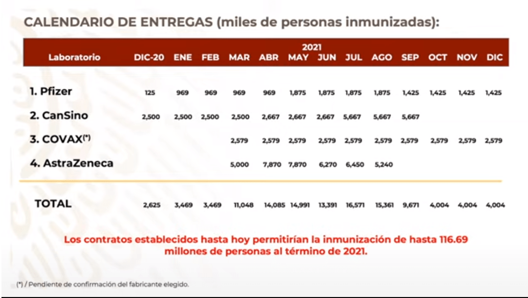
On October 13 2020, the Mexican government announced a vaccine delivery plan from Pfizer-BioNTech and other companies as part of the COVID-19 vaccination campaign.

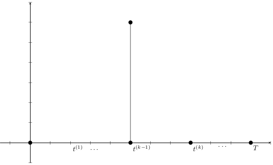
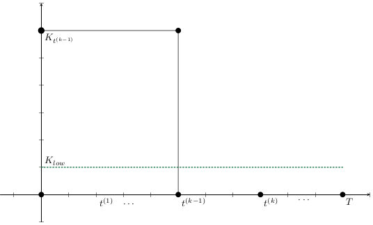
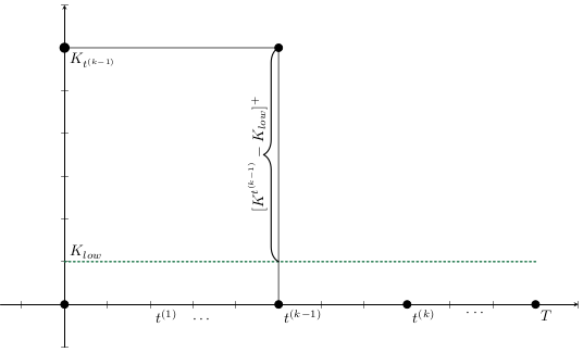
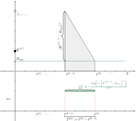
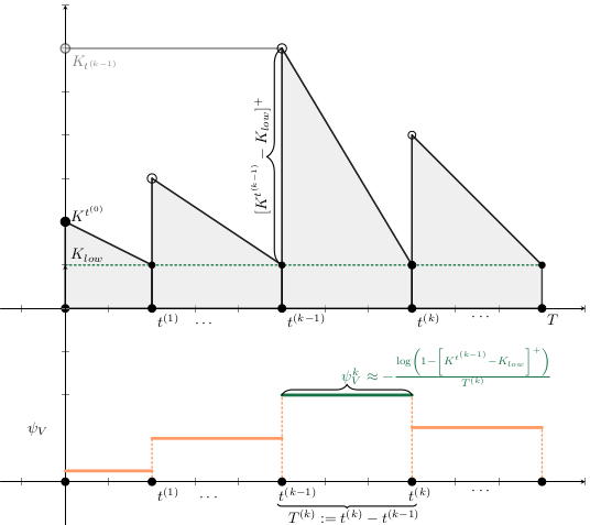
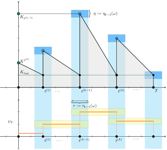
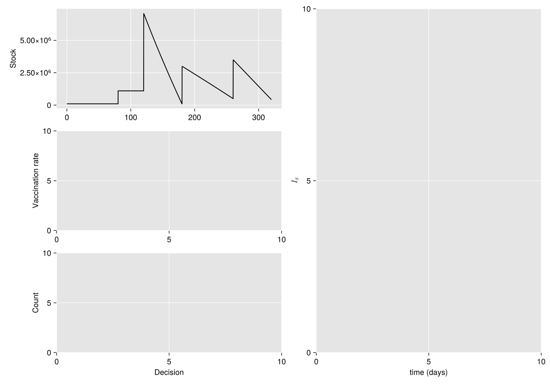
Methods. Given a vaccine shipping schedule, we describe stock management with a backup protocol and quantify the random fluctuations due to a program under high uncertainty.

Then, we incorporate this dynamic into a system of ODE that describes the disease and evaluate its response.

Nonlinear control: HJB and DP

Given

\frac{dx}{dt} = f(x(t))

Goal:

Desing

to follow

s. t. optimize cost

\text{action } a_t\in \mathcal{A},

\text{state } x_t

\frac{dx_{t}}{dt} =f(x_{t} ,a_{t})

Agent

a_t\in \mathcal{A}

x_t

J(x_t, a_t, 0, T) = Q(x_T, T) + \int_0^T \mathcal{L}(x_{\tau}, a_{\tau}) d_{\tau}

J(x_t, a_t, 0, T) .

Nonlinear control: HJB and DP

V(x_0, 0, T):= \min_{a_t \in \mathcal{A}} J(x_t, a_t, 0, T)

V(x_0, 0, T) = V(x_0, 0, t) + V(x_0, t, T)

Bellman optimality principle

Control Problem

\frac{dx_t}{dt} = f(x_t, a_t)

\min_{a_t\in \mathcal{A}} J(x_t, a_t, 0, T) = Q(x_T, T) + \int_0^T \mathcal{L}(x_{\tau}, a_{\tau}) d_{\tau}

s.t.

x_T

x_t

x_0

\frac{\partial V}{\partial t} = \min_{a_t\in \mathcal{A}} \left[ \left( \frac{\partial V}{\partial x} \right)^{\top} f(x,a) + \mathcal{L}(x,a) \right]

\begin{equation*} \begin{aligned} S'(t) &= -\beta IS \\ I'(t) &= \beta IS - \gamma I \\ R'(t) & = \gamma I \\ & S(0) = S_0, I(0)=I_0, R(0)=0 \\ & S(t) + I(t) + R(t )= 1 \end{aligned} \end{equation*}

\lambda_V:= \underbrace{ \textcolor{orange}{\xi}}_{cte.} \cdot \ S(t)

\begin{equation*} \begin{aligned} S'(t) &= -\beta IS - \textcolor{red}{\lambda_V(t)} \\ I'(t) &= \beta IS - \gamma I \\ R'(t) & = \gamma I \\ V'(t) & = \textcolor{red}{\lambda_V(t)} \\ & S(0) = S_0, I(0)=I_0, \\ &R(0)=0, V(0) = 0 \\ & S(t) + I(t) + R(t) + V(t)= 1 \end{aligned} \end{equation*}

\begin{equation*} \begin{aligned} S'(t) &= -\beta IS - \textcolor{red}{\lambda_V(x, t)} \\ I'(t) &= \beta IS - \gamma I \\ R'(t) & = \gamma I \\ V'(t) & = \textcolor{red}{\lambda_V(x,t)} \end{aligned} \end{equation*}

\lambda_V:= \underbrace{ \textcolor{orange}{\Psi_V}}_{cte.} \cdot \ S(t)

\begin{aligned} S'(t) &= \cancel{-\beta IS} - \underbrace{\textcolor{red}{\lambda_V(x, t)}}_{=\Psi_V S(t)} \\ I'(t) &= \cancel{\beta IS} - \cancel{\gamma I} \\ {R'(t)} & = \cancel{\gamma I} \\ V'(t) & = \underbrace{\textcolor{red}{\lambda_V(x, t)}}_{=\Psi_V S(t)} \\ & S(0) \approx 1, I(0) \approx 0, \\ &R(0)\approx 0, V(0) = 0 \\ & S(t) + \cancel{I(t)} + \cancel{R(t)} +\cancel{ V(t)}= 1 \end{aligned}

\begin{aligned} S'(t) &= - \Psi_V S(t) \\ V'(t) & = \Psi_V S(t) \\ & S(0) \approx 1, V(0) = 0 \\ & S(t) + V(t) \approx 1 \end{aligned}

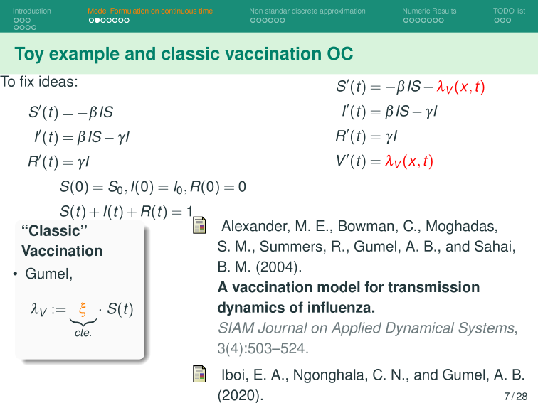
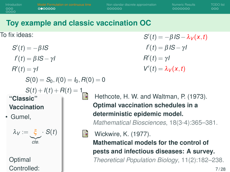
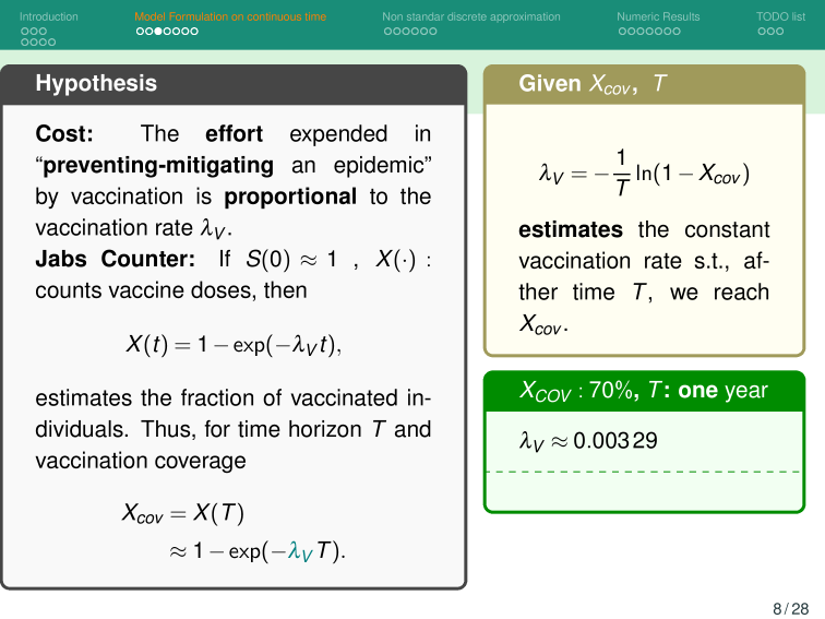
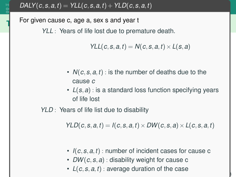
The effort invested in preventing or mitigating an epidemic through vaccination is proportional to the vaccination rate

\textcolor{orange}{\Psi_V}

Let us assume at the beginning of the outbreak:

\textcolor{orange}{S(0)\approx 1}

\begin{aligned} S'(t) &= - \Psi_V S(t) \\ V'(t) & = \Psi_V S(t) \\ & S(0) \approx 1, V(0) = 0 \\ & S(t) + V(t) \approx 1 \end{aligned}

S(t) \approx N \exp(-\Psi_V t)

\begin{aligned} V(t) \approx \cancel{V(0)} + \int_0^t \Psi_V S(\tau) d\tau \end{aligned}

\begin{aligned} V(t) &\approx \cancel{V(0)} + \int_0^t \Psi_V S(\tau) d\tau \\ & \approx \int_0^t N \Psi_V \exp(-\Psi_V \tau) d\tau \\ & \approx N \exp(-\Psi_V \tau) \mid_{\tau=t}^{\tau=0} \\ &= \cancel{N} \exp(1 - \exp(-\Psi_V t)) \end{aligned}

Then we estimate the number of vaccines with

X_{vac}(t) := \int_{0}^t \Psi_v \Bigg( \underbrace{S(\tau)}_{ \substack{ \text{target} \\ \text{pop.} } }\Bigg )

Then, for a vaccination campaign, let:

\begin{aligned} \textcolor{orange}{T}: &\text{ time horizon} \\ \textcolor{green}{ X_{cov}:= X_{vac}(} \textcolor{orange}{T} \textcolor{green}{)}: &\text{ covering at time $T$} \end{aligned}

\begin{aligned} X_{cov} = &X_{vac}(T) \\ \approx & 1 - \exp(-\textcolor{teal}{\Psi_V} T). \\ \therefore & \textcolor{teal}{\Psi_V} = -\frac{1}{T} \ln(1 - X_{cov}) \end{aligned}

Then we estimate the number of vaccines with

X_{vac}(t) := \int_{0}^t \Psi_v \Bigg( \underbrace{S(\tau)}_{ \substack{ \text{target} \\ \text{pop} } }\Bigg )

Then, for a vaccination campaign, let:

\begin{aligned} \textcolor{orange}{T}: &\text{ horizon time} \\ \textcolor{green}{ X_{cov}:= X_{vac}(} \textcolor{orange}{T} \textcolor{green}{)}: &\text{ Coverage at time $T$} \end{aligned}

\begin{aligned} X_{cov} = &X_{vac}(T) \\ \approx & 1 - \exp(-\textcolor{teal}{\Psi_V} T). \\ \therefore & \textcolor{teal}{\Psi_V} = -\frac{1}{T} \ln(1 - X_{cov}) \end{aligned}

Estimated population of Hermosillo, Sonora in 2024 is 930,000.

So to vaccinate 70% of this population in one year:

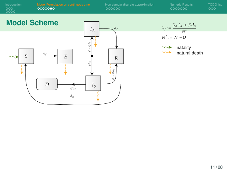
\begin{aligned} 930,000 &\times 0.00329 \\ \approx & 3,059.7 \ \text{dósis/día} \end{aligned}

Base Model

\begin{align*} L^{t_{n+1}^{(k)}} &= K^{t_{n}^{(k)}} \cdot \left( 1 - e^{ - \textcolor{orange}{\lambda(T^{t_{n}^{(k)}})} \cdot t_{n}^{(k)} } \right), \\ \lambda(T^{t_{n+1}^{(k)}}) &= \kappa \cdot \max\{0, \ \textcolor{orange}{T^{t_{n}^{(k)}}} - \mu_{T}\}, \end{align*}

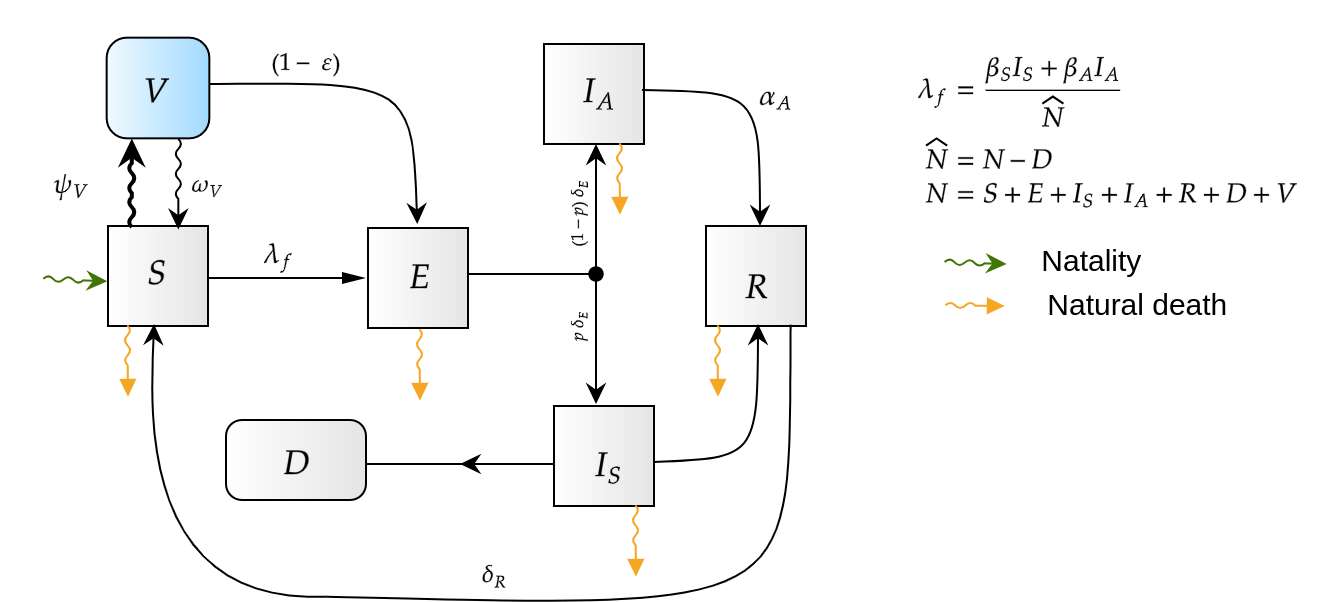
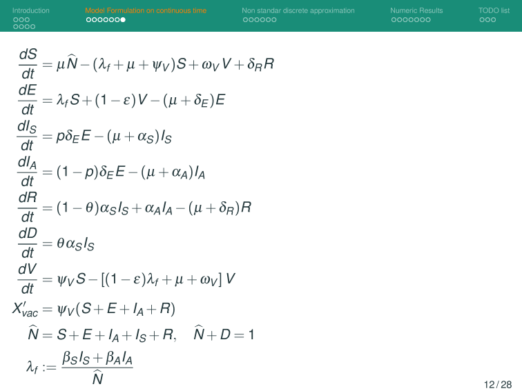
Stock degradation due to Temperature

d\textcolor{orange}{T_t} = \theta_T (\mu_T - T_t) dt + \sigma_T dW_t

\begin{align*} X_{vac}^{t_{n+1}^{(k)}} &= \varphi(h_k)\psi_V^{(k)} \left( S^{t_{n}^{(k)}} + E^{t_{n}^{(k)}} + I_A^{t_{n}^{(k)}} + R^{t_{n}^{(k)}} \right) + X_{vac}^{t_{n}^{(k)}}, \\ K^{t_{n+1}^{(k)}} &= \max \left\{ 0, \left( K^{t_n^{(k)}} - K_{low} \right) - (X_{vac}^{t_{n+1}^{(k)}} - X^{t_0^{(k)}}_{vac}) - \textcolor{orange}{ L^{t_{n}^{(k)}}} \right\}, \end{align*}

\begin{aligned} %C_{t+1} &= C(x_{t}, a_{t}) \\ %\Phi_{t+1}^{h}(x_t,a_t) &= x_t +\varphi(h,\theta) \end{aligned}

Agent

R_{t+1}

x_{t+1}

x_0,a_0,R_1,

a_t\in \mathcal{A}(x_t)

action

state

x_{t}

reward

R_{t}

x_0, a_0, R_1, x_1, a_1, R_2, \cdots, x_t, a_t, R_{t+1} \cdots, x_{T-1}, a_{T-1}, R_T, x_T

G_t := R_{t+1} + \cdots + R_{T-1} + R_{T}

\begin{aligned} G_t &:= R_{t+1} + \gamma R_{t+2} + \gamma^2 R_{t+3}+ \cdots \\ &= \sum_{k=0} \gamma^{k} R_{t+1+k}, \qquad \gamma \in [0,1] \end{aligned}

\begin{aligned} x_{t_{n+1}} & = x_{t_n} + F(x_{t_n}, \theta, a_0) \cdot h, \quad x_{t_0} = x(0), \\ \text{where: }& \\ t_n &:= n \cdot h, \quad n = 0, \cdots, N, \quad t_{N} = T. \end{aligned}

\begin{aligned} &\min_{a_{0}^{(k)} \in \mathcal{A}_0} c(x_{\cdot}, a_0):= c_1(a_0^{(k)})\cdot T^{(k)} + \sum_{n=0}^{N-1} c_0(t_n, x_{t_n}) \cdot h \\ \text{ s.t.} & \\ & x_{t_{n+1}} = x_{t_n} + F(x_{t_n}, \theta, a_0) \cdot h, \quad x_{t_0} = x(0), \\ \text{where: }& \\ t_n &:= n \cdot h, \quad n = 0, \cdots, N, \quad t_{N} = T. \end{aligned}

\begin{aligned} C(x_{t^{(k+1)}}, & a_{t^{(k+1)}}) = \\ & C_{YLL}(x_{t^{(k+1)}},a_{t^{(k+1)}}) \\ +& C_{YLD}(x_{t^{(k+1)}},a_{t^{(k+1)}}) \\ +& C_{stock}(x_{t^{(k+1)}},a_{t^{(k+1)}}) \\ +& C_{campaign}(x_{t^{(k+1)}},a_{t^{(k+1)}}) \end{aligned}

J(x,\pi) = E\left[ \sum_{k=0}^M C(x_{t^{(k)}},a_{t^{(k)}}) | x_{t^{(0)}} = x , \pi \right]

\begin{aligned} C_{YLL}(x_{t^{(k+1)}},a_{t^{(k+1)}}) &= \int_{t^{(k)}}^{t^{(k+1)}} YLL dt, \\ C_{YLD}(x_{t^{(k+1)}},a_{t^{(k+1)}}) &= \int_{t^{(k)}}^{t^{(k+1)}} YLD(x_t, a_t) dt \\ YLL(x_t, a_t) &:= m_1 p \delta_E (E(t) - E^{t^{(k)}} ), \\ YLD(x_t, a_t) &:= m_2 \theta \alpha_S(E(t) - E^{t^{(k)}}), \\ t &\in [t^{(k)},t^{(k + 1)}] \end{aligned}

\begin{aligned} C_{stock}(x_{t^{(k+1)}},a_{t^{(k+1)}}) & = \int_{t^{(k)}}^{t^{(k+1)}} m_3(K_{Vac}(t) - K_{Vac}^{t^{(k)}}) dt \\ C_{campaign}(x_{t^{(k+1)}},a_{t^{(k+1)}}) &=\int_{t^{(k)}}^{t^{(k+1)}} m_4(X_{vac}(t) - X_{vac}^{t^{(k)}}) dt \end{aligned}