Quantum algorithms for machine learning
Soutenance de thése de
Alessandro Luongo
20 Novembre 2020
Supervisor: Iordanis Kerenidis
Co-supervisor: Frédéric Magniez.
aluongo@irif.fr

This thesis addresses this question:
Is machine learning a promising domain for quantum algorithms*?
* to be run on fault-tolerant quantum computers with quantum access to classical data
Runtime
\( O\left(nd^2 \right) \)
\( O\left(\|X\|_0 \textcolor{red}{\times} \text{poly}( \kappa(X), \epsilon, ...) \right) \)
\( O\left(\|X\|_0 \textcolor{red}{+} \text{poly}(\kappa(X), \epsilon, \mu(X), ...) \right) \)
Worst-case classical algorithms
Randomized classical algorithms
Input \( X \in \mathbb{R}^{n \times d} \text{ with } n \gg d\)
Quantum algorithms

This thesis addresses this question:
Is machine learning a promising domain for quantum algorithms*?
Runtime
\( O\left(nd^2 \right) \)
Worst-case classical algorithms
Randomized classical algorithms
Quantum algorithms
Input \( X \in \mathbb{R}^{n \times d} \text{ with } n \gg d\)


\( O\left(\|X\|_0 \right) \textcolor{red}{+} O\left( \text{poly}(\kappa(X), \epsilon, \mu(X), ...) \right) \)
* to be run on fault-tolerant quantum computers with quantum access to classical data
\( O\left(\|X\|_0 \textcolor{red}{\times} \text{poly}( \kappa(X), \epsilon, ...) \right) \)

The end of Moore's law?
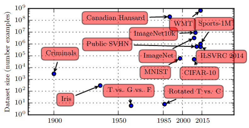
Size of benchmark datasets over time
GB range: 52.8% (2013), 54.3% (2014),
55.6% (2015) 56.0% (2018)
What was the largest dataset you analyzed?
https://www.kdnuggets.com/2018/10/poll-results-largest-dataset-analyzed.html
Quantum!

-
Quantum classification of the MNIST dataset via slow feature analysis. I. Kerenidis, AL - PRA. [QSFA] (supervised ML, dimensionality reduction, classification, experiments on real data)
-
q-means: A quantum algorithm for unsupervised machine learning.
I. Kerenidis, J. Landman, AL, A. Prakash - NeurIPS2019 [QMEANS] (unsupervised ML, clustering, experiments on real data)
-
Quantum Expectation-Maximization for Gaussian mixture models.
I. Kerenidis, AL, A. Prakash - ICML2020 [QEM] (unsupervised ML, clustering, experiments on real data)
-
Quantum algorithms for spectral sums. C. Shao, AL - arXiv:2011.06475 [QSS] (quantum algorithms numerical linear algebra)
-
Application of quantum algorithms for spectral sums. AL - (to appear) [AQSS] (statistics, applications.)
Contributions
Quantum classification of the MNIST dataset via slow feature analysis. I. Kerenidis, AL - PRA. [QSFA] (supervised ML, dimensionality reduction, classification, experiments on real data)
-
q-means: A quantum algorithm for unsupervised machine learning.
I. Kerenidis, J. Landman, AL, A. Prakash - NeurIPS2019 [QMEANS] (unsupervised ML, clustering, experiments on real data)
-
Quantum expectation-maximization for Gaussian mixture models.
I. Kerenidis, AL, A. Prakash - ICML2020 [QEM] (unsupervised ML, clustering, experiments on real data)
Quantum algorithms for spectral sums. C. Shao, AL - arXiv:2011.06475 [QSS] (quantum algorithms numerical linear algebra)
Application of quantum algorithms for spectral sums. AL - (to appear) [AQSS] (statistics, applications.)
Quantum algorithms for data representation. A. Bellante, AL - (to appear) [QADR] (natural language processing, experiments on real data, eigenvalue problems)
Contributions
The QML toolkit
-
Query access to matrices
-
Quantum linear algebra
-
Distance estimations
-
Singular Value Estimation
-
Tomography (of pure states)
-
Hamiltonian simulation
-
Amplitude estimation and amplification
-
Singular value transformations
-
Polynomial approximations
-
...
Quantum access to a matrix
-
Classical preprocessing time: \( O(\textcolor{red}{nd} \log nd) \)
-
Classical space: \( O\left( \textcolor{red}{nd} \log nd \right) \)
-
Query time: \( O(\textcolor{red}{\log nd}) \)
-
Quantum space: \( O \left(\textcolor{red}{ \log nd }\right) \)
Iordanis Kerenidis, Anupam Prakash - 8th Innovations in Theoretical Computer Science Conference - ITCS 2017.
Anupam Prakash - Quantum algorithms for linear algebra and machine learning. Diss. UC Berkeley - 2014.
Quantum query:
\( |i\rangle |0 \rangle \mapsto |i\rangle |x_i\rangle \)
Where \(|x_i\rangle=\frac{1}{\|x_i\|_2} x_i = \frac{1}{\|x_i\|_2} \sum_i (x_i)_j |j\rangle \)
\( X \in \mathbb{R}^{\textcolor{red}{n \times d}} = [x_1, \dots, x_n]^T \) \( x_i \in \mathbb{R}^d\)
-
Classical preprocessing time: \( O(\textcolor{red}{nd} \log nd) \)
-
Classical space: \( O\left( \textcolor{red}{nd} \log nd \right) \)
-
Query time: \( O(\textcolor{red}{\log nd}) \)
-
Quantum space: \( O \left(\textcolor{red}{ \log nd }\right) \)
Iordanis Kerenidis, Anupam Prakash - 8th Innovations in Theoretical Computer Science Conference - ITCS 2017.
Anupam Prakash - Quantum algorithms for linear algebra and machine learning. Diss. UC Berkeley - 2014.
Where \(|x_i\rangle=\frac{1}{\|x_i\|_2} x_i = \frac{1}{\|x_i\|_2} \sum_i (x_i)_j |j\rangle \)
Quantum query:
\( \frac{1}{\sqrt{n}}\sum_i |i\rangle |0 \rangle \mapsto \frac{1}{\sqrt{n}}\sum_i |i\rangle |x_i\rangle \)
\( X \in \mathbb{R}^{\textcolor{red}{n \times d}} = [x_1, \dots, x_n]^T \) \( x_i \in \mathbb{R}^d\)
Quantum access to a matrix
Quantum linear systems of equations
Given:
-
quantum sparse access \(A \in \R^{n \times n}\),
-
and a vector \(x \in \R^n\)
The HHL algorithm produces a state \(|z\rangle\) such that
\( \kappa(A) = \frac{\sigma_1(A)}{\sigma_n(A)} \) and \( s = \text{row's sparsity} \)
Harrow, Aram, Avinatan Hassidim, Seth Lloyd - Physical review letters - 2009
Quantum linear systems of equations
The HHL algorithm produces a state \(|z\rangle\) such that
\( \kappa(A) = \frac{\sigma_1(A)}{\sigma_n(A)} \)
Harrow, Aram, Avinatan Hassidim, Seth Lloyd - Physical review letters - 2009
Given:
-
quantum access \(A \in \R^{n \times n}\),
-
and a vector \(x \in \R^n\)
Given quantum access to a (sparse) \(A \in \R^{n \times n}\), and a vector \(x \in \R^n\)
The HHL algorithm produces a state \(|z\rangle\) such that
Harrow, Aram, Avinatan Hassidim, Seth Lloyd - Physical review letters - 2009
Quantum linear systems of equations
\( \kappa(A) = \frac{\sigma_1(A)}{\sigma_n(A)} \)
\( s = \text{row's sparsity} \)
Quantum singular value transformations
Given matrix \(A \in \R^{n \times m}\), and a vector \(x \in \R^m\)
It is possible to produce a state \(|z\rangle\) s.t.
In general:
\(f(A) = \sum_i^d f(\sigma_i)|u_i\rangle \langle v_i| \)
Iordanis Kerenidis, Anupam Prakash - 8th Innovations in Theoretical Computer Science Conference - 2017.
András Gilyén, et al. - Proceedings of the 51st Annual ACM SIGACT Symposium on Theory of Computing - 2019.
Guang Hao Low, Isaac L. Chuang - Physical review letters - 2017.
\(\mu(A) = \min\left(\|A\|_F, \sqrt{\max_{i \in [n]} \|a_i\|_{2p}^{2p} \max_{i \in [d]} \|a_{*i}\|_{2(1-p)}^{(1-p)} }\right) \)
Distance estimation subroutines
-
Euclidean distance [QMEANS]
-
Quadratic forms [Thesis]
-
Distance induced by \(A\) [QEM]
\(|i,j\rangle \mapsto |i,j ,\|x_i- x_j\|_2\rangle \)
\(|i,j\rangle \mapsto |i,j ,d_A(x_i, x_j) \rangle \)
\(|i,j\rangle \mapsto |i,j ,x_i^TA^\textcolor{orange}{-1}x_j \rangle \)
\( \widetilde{O}(\frac{1 }{\epsilon} ) \)
\( \widetilde{O}(\frac{\mu(A)}{\epsilon} ) \)
\( \widetilde{O}(\frac{\mu(A)\textcolor{orange}{\kappa(A)}}{\epsilon} ) \)
\( X \in \mathbb{R}^{n \times d} = [x_1, \dots, x_n]^T \) \( x_i \in \mathbb{R}^d\)
We can produce an estimate \(\overline{x}\) of \(|x\rangle\) such that \(\|\overline{x}\| = 1\) and
using
Tomography of pure states
Iordanis Kerenidis, Anupam Prakash - ACM Transactions on Quantum Computing, 2020.
Iordanis Kerenidis, Anupam Prakash, Jonas Landman - International Conference on Learning Representations, 2019.
samples
using
samples
SVE of product of matrices
Theorem: Assume to have quantum access to \(A, B \in \mathbb{R}^{n \times n} \).
There is an algorithm that performs the mapping
\( \sum_i \alpha_i |i\rangle \mapsto \sum_i \alpha_i|i, \sigma_i \rangle \)
where \(\sigma_i \) is the i-th singular value of \(AB\) in time
\(O\left(\frac{(\kappa(A)+\kappa(B))( \mu(A)+\mu(B))}{\epsilon}\right) \)
Shantanav Chakraborty., et al. - 46th International Colloquium on Automata, Languages, and Programming - 2019.
[QSFA]
Supervised
Learning
-
\(X \in \mathbb{R}^{n \times d} \) dataset
-
\( L \in [K]^{n} \) labels
(classification)
Quantum supervised learning
-
Quantum slow feature analysis for dimensionality reduction
-
Quantum Frobenius distance classifier: a simple NISQ classifier
-
Simulation on MNIST dataset of handwritten digits
-
Extension to other generalized eigenvalue problems in ML
[QSFA, Thesis]

https://cmp.felk.cvut.cz/cmp/software/stprtool
Slow Feature Analysis
\(X \in \mathbb{R}^{n \times \textcolor{orange}{d}} \) (images)
\(Y \in \mathbb{R}^{n \times \textcolor{orange}{K}} \)
\( y_i =\left[ w_1^Tx_i, \dots, w_K^Tx_i\right] \)
\( \langle Y_{*j}\rangle =0 \)
\( \langle Y^2_{ij}\rangle = 1 \)
\( \forall j' < j : \langle Y_{*j'} Y_{*j} \rangle = 0 \)
\(L \in [K]^{n} \) (labels)
Finding the model \( \{w_j\}_{j=1}^K \) reduces to a constrained optimization problem:
-
The componentwise average should be zero.
-
The componentwise variance should be \(1\).
-
Signals are maximally uncorrelated.
Constraints
Slow Feature Analysis
\( \Delta_j = \frac{1}{a} \sum_{j=1}^K \sum (w_j^Tx^{(j)}_s - w_j^Tx^{(j)}_t)^2 \)
\(X \in \mathbb{R}^{n \times \textcolor{orange}{d}} \) (images)
\(Y \in \mathbb{R}^{n \times \textcolor{orange}{K}} \)
\( y_i =\left[ w_1^Tx_i, \dots, w_K^Tx_i\right] \)
\(L \in [K]^{n} \) (labels)
Finding the model \( \{w_j\}_{j=1}^K \) reduces to an optimization problem:
\(\substack{s,t \in T_k \\ i<j}\)

Quantum Slow Feature Analysis
Theorem:
-
Quantum access to \(X\), derivative matrix \(\dot{X}\)
-
Let \( \epsilon, \theta, \delta, \eta >0\)
There are quantum algorithms to get:
-
Map dataset in the slow feature space \( |\overline{Y}\rangle \) in time: $$ \tilde{O}\left( \frac{ ( \kappa(X) + \kappa(\dot{X})) ( \mu({X})+ \mu(\dot{X}) ) }{\delta\theta} \gamma_{K-1} \right) $$
-
Find \( \{ w_j\}_{j=0}^{K}\) in time: $$O\left(d^{1.5}\sqrt{K}\frac{\kappa(X)\kappa(\dot X X)(\mu(X) + \mu(\dot{X}))}{\epsilon^2}\right)$$
[QSFA]
QFDC: classification in slow feature space
Theorem: Assume to have quantum access to \(|Y\rangle\) in time T, we can label images in \(k\) classes in time \(O(\frac{kT}{\epsilon}) \).
Definition: QFDC (Quantum Frobenius distance classifier):
A point is assigned to the cluster with smallest
normalized--average-squared distance
between the point and the points of the cluster.
[QSFA]
We get high accuracy with a fast quantum classifier

Classification of handwritten digits of MNIST dataset
Ex: polynomial expansion
of degree 2:
\([x_1, x_2, x_3] \mapsto [x_1^2, x_1x_2 \dots x_3^3 ]\)
We get high accuracy with a fast quantum classifier
Malware detection via DGA classification
| Accuracy | Original classifier | With slow-feature |
|---|---|---|
| Logistic Regression | 89% | 90.5% (+1.5%) |
| Naive Bayes classifier | 89.3% | 92.3% (+3%) |
| Decision Trees | 91.4% | 94.0% (+2.6%) |
[Thesis]
-
Using SFA in a classification problem improves its accuracy
-
QSFA can process old datasets in new ways!
SFA as instance of a more general problem
The GEP (Genrealized Eigenvalue Problem) is defined as:
- \(B=X^TX\)
- \(A=\dot X^T \dot X \)
In SFA:
-
ICA Independent Component Analysis
-
G-IBM Gaussian Information Bottleneck Method
-
CCA Canonical Correlation Analysis
-
SC (some) Spectral Clustering [1]
-
PLS Partial Least Squares
-
LE Laplacian Eigenmaps
-
FLD Fisheral Linear Discriminant
-
SFA Slow Feature Analysis
-
KPCA Kernel Principal Component Analysis
\( AW = BW\Lambda \)
[1] Iordanis Kerenidis, Jonas Landman - Quantum spectral clustering. arXiv2007.00280. (2020)
Quantum supervised learning
-
Quantum slow feature analysis for dimensionality reduction
-
Simulation on MNIST dataset of handwritten digits
-
Quantum Frobenius distance classifier: a simple NISQ classifier
-
Extension to other generalized eigenvalue problems in ML
[QSFA, Thesis]
Unsupervised
Learning
-
\(X \in \mathbb{R}^{n \times d} \)
(clustering)
Quantum unsupervised
learning
-
q-means for clustering (quantum version of k-means)
-
Quantum Expectation-Maximization
-
Simulation on VoxForge dataset for speaker recognition
The k-means algorithm:
\( t \leftarrow 0 \)
Step 1:
-
Compute distance for all points \(x_i \) and centroid \(\mu_j^{t}, \) $$ d(x_i, \mu_j^{t}) $$
-
Assign points to closest cluster: $$ l(x_i) = \argmin_{c \in [K]}{ d(x_i, \mu_j^{t})}$$
Step 2:
-
Compute the barycenter: $$\mu_j^{t+1} = \frac{1}{|C_j|}\sum_{i \in C_j}^{} x_i $$
t \(\leftarrow \)t+1
\(O(tkdn) \)
q-means
\( t \leftarrow 0 \)
Step 1:
-
Compute distance for all points \(v_i \) and centroid \(\mu_j^{t}, \) $$|i,j\rangle \mapsto |i,j,d(v_i, \mu_j^{t})\rangle $$
-
Generate characteristic vector of a cluster: $$ |\chi_j \rangle = \frac{1}{|C_j|}\sum_{i \in C_j} |i \rangle$$
Step 2:
-
Use quantum linear algebra to build $$|\mu_j^{t+1}\rangle = \frac{1}{|C_j|}\sum_{i \in C_j}^{} |v_i\rangle $$
-
Perform tomograph on \( |\mu_j^{t+1}\rangle \)
-
Build quantum access to \( \mu_j\).
\( t \leftarrow t+1 \)
q-means
Theorem: Given quantum access to a matrix \(X \in \mathbb{R}^{n \times d} \), there is quantum algorithm that fits a k-means model in time:
\( \widetilde{O}\left( k^2 d \frac{\eta^{2.5}}{\delta^3} \right) \)
Classical: \( O\left(\textcolor{red}{n}kd\right) \)
[QMEANS]
\( \| \mu_j - \mu_j^* \| \leq \delta \)
\( \eta = \max_i (\|x_i\|^2 ) \)
k-means learns the cluster's barycenters
\( \{\mu_j\}_{j=1}^K = \text{argmin} \sum_i^n d(x_i, \mu_{l(x_i)} \))
For a dataset \( \{ x_i \}_{i}^n \) finds centroids \(\{ \mu_j\}_{j=1}^K\) such that:
Text
i.e. minimize distance between points and their cluster's barycenter.
q-means
\( t \leftarrow 0 \)
Expectation:
-
Compute distance for all points \(v_i \) and centroid \(\mu_j^{t}, \) $$|i,j\rangle \mapsto |i,j,d(v_i, \mu_j^{t})\rangle $$
-
Generate characteristic vector of a cluster: $$ |\chi_j \rangle = \frac{1}{|C_j|}\sum_{i \in C_j} |i \rangle$$
Maximization:
-
Use quantum linear algebra to build $$|\mu_j^{t+1}\rangle = \frac{1}{|C_j|}\sum_{i \in C_j}^{} |v_i\rangle $$
-
Perform tomograph on \( |\mu_j^{t+1}\rangle \)
-
Build quantum access to \( \mu_j\).
\( t \leftarrow t+1 \)
Gaussian mixture models
\( k \) labels
Multinomial distribution
\( [\theta, \mu_1, \dots, \mu_k, \Sigma_1, \dots, \Sigma_k ] \)
\( \gamma^* = \text{argmax} \prod_i \sum_{j \in [k]} \theta_j p(x_i|\mu_j,\Sigma_j) \)
Gaussian distribution
\(_\gamma\)
- \(\|\theta-\overline{\theta}\|<\delta_\theta \)
- \(\|\mu_j - \overline{\mu_j}\| < \delta_\mu \)
- \(\|\Sigma_j - \overline{\Sigma_j}\| < \delta_\mu\sqrt{\eta}\)
Error introduced by quantum algorithm parameters
Maximum Likelihood Estimation
Expectation-Maximization
Repeat
\(t = 0\)
- Expectation \[ r_{ij}^t \leftarrow \frac{\theta^t_j N(v_i; \mu^t_j, \Sigma^t_j )}{\sum_{l=1}^k \theta^t_l N(v_i; \mu^t_l, \Sigma^t_l)}\]
\( t \leftarrow t+1 \)
Until \( | \ell(\gamma^{t-1};V) - \ell(\gamma^t;V) | < \tau \)
- Maximization
-
Update the parameters \(\theta, \mu, \Sigma \) using the responsibilities \(r_{ij} \)
Quantum Expectation-Maximization
Repeat
\(t = 0\)
\( t \leftarrow t+1 \)
Until \( | \ell(\gamma^{t-1};V) - \ell(\gamma^t;V) | < \tau \)
- Maximization
-
Use \(U_R \) to generate states proportional to \(\theta^{t+1}, \mu^{t+1}, \Sigma^{t+1} \)
-
Perform tomography and create quantum access.
-
Create mapping \[ U_R |i,j\rangle|0\rangle \mapsto |i,j\rangle |r_{ij} ^t\rangle \]
- Expectation
Quantum Expectation-Maximization
Repeat
- Expectation \[ |r_{ij}^t\rangle \leftarrow \frac{\theta^t_j N(v_i; \mu^t_j, \Sigma^t_j )}{\sum_{l=1}^k \theta^t_l N(v_i; \mu^t_l, \Sigma^t_l)}\]
- Maximization
\( |\theta_j^{t+1}\rangle \leftarrow \frac{1}{n}\sum_{i=1}^n r^{t}_{ij} \)
\( |\mu_j^{t+1}\rangle \leftarrow \frac{\sum_{i=1}^n r^{t}_{ij} v_i }{ \sum_{i=1}^n r^{t}_{ij}}\)
\( |\Sigma_j^{t+1}\rangle \leftarrow \frac{\sum_{i=1}^n r^{t}_{ij} (v_i - \mu_j^{t+1})(v_i - \mu_j^{t+1})^T }{ \sum_{i=1}^n r^{t}_{ij}} \)
\( t \leftarrow t+1\)
Until \( | \overline{\ell(\gamma^{t-1};V)} - \overline{\ell(\gamma^t;V)} | < \tau \)
Quantum Expectation-Maximization
Repeat
- Expectation \[ r_{ij}^t \leftarrow \frac{\theta^t_j N(v_i; \mu^t_j, \Sigma^t_j )}{\sum_{l=1}^k \theta^t_l N(v_i; \mu^t_l, \Sigma^t_l)}\]
- Maximization
Update the parameters \(\theta, \mu, \Sigma \) using the responsibilities \(r_{ij} \)
\( t \leftarrow t+1 \)
Until \( | \ell(\gamma^{t-1};V) - \ell(\gamma^t;V) | < \tau \)
Quantum Expectation-Maximization for
Gaussian mixture models
Theorem: Given quantum access to a matrix \( X \in \mathbb{R}^{n \times d} \) there is a quantum EM algorithm that fits a GMM in time:
[QEM]
Classical: \( O(d^2 k n) \)
\( O\left( d^2k^{4.5} \gamma(X)\textcolor{red}{\log n}\right) \) \(\gamma(n)= O\left( \frac{\eta^3 \kappa(X)\kappa^2(\Sigma)\mu(\Sigma)\mu(X)}{\delta^3} \right) \)

We get high accuracy with a fast quantum classifier
-
Classical ML accuracy: 169/170
-
Quantum ML accuracy: 167/170
-
Max element of \( \Sigma_j^{-1}\) set to \(5\) via \(\kappa = \frac{1}{\lambda_\tau} \)

Speaker recognition problem on VoxForge dataset
Quantum unsupervised
learning
-
q-means for clustering (quantum version of k-means)
-
Quantum Expectation-Maximization
-
Simulation on VoxForge dataset for speaker recognition
Quantum Spectral Sums
\(S_f(A) = \sum_i^n f(\lambda_i) \)
\(S_f(A) = \sum_i^n f(\sigma_i) \)
\(A \in \mathbb{R}^{n \times n} \) SPD
\( f : \mathbb{R} \mapsto \mathbb{R} \)
Theorem: Quantum access to a SPD matrix \( A \),
\(\|A\| < 1 \) and \(\epsilon \in(0,1)\).
There is a quantum algorithm that estimate \( \log\det(A)\) with relative error \(\epsilon \) w.h.p. in time \( \widetilde{O}({\mu(A) \kappa(A)}/{\epsilon})\).
Quantum algorithms for log-determinant
\( S_{\log(x)}(A) =\log\det(A) = \sum_i^n \log(\lambda_i) \)
Application: Tyler's M-estimator.
[QSS]
Tyler's M-estimator
\(\Gamma_* \leftarrow \frac{1}{n} \sum_{i=1}^n \frac{x_ix_i^T}{x_i^T\Gamma_*^{-1}x_i} \)
-
Data from sub-Gaussian distributions.
-
Robust to outliers
-
Valid for data \( X^{n \times d}\) with \( n,d \mapsto \infty \)
[Thesis, AQSS]
In many cases \(C = X^TX\) is not a "good" sample covariance matrix
Tyler's M-estimator
[Thesis, AQSS]
Goes, J, et al. - The Annals of Statistics 2020.
Might benefits from componentwise thresholding:
Runtime:
\[ \tilde O\left(\textcolor{red}{d^2}\frac{\mu(X)\kappa(\Sigma_k)\mu(\Sigma_k)}{\epsilon^3}\gamma\right) \]
\( \Gamma_{k+1} = \sum_{i=1}^n \frac{x_ix_i^T}{ x_i^T \Gamma_k^{-1}x_i}/ Tr[\sum_{i=1}^n \frac{x_ix_i^T}{x_i^T \Gamma_k^{-1}x_i}]\)
Stopping condition: log-likelihood with a log-determinant
Classical:
\( O\left( d^2n \right) \)
Other spectral sums and applications (not in thesis)
-
Schatten p-norm \(O(2^{p/2}\mu(A)(p+\kappa(A))\sqrt{n}/\epsilon) \)
-
Von Neumann entropy \(O(\mu(A)\kappa(A)n /\epsilon )\)
-
Trace of Inverse \(O(\mu^2 \kappa(A)^2/\epsilon) \)
Applications..
-
Counting number of spanning trees
-
Counting triangles
-
Estimating effective resistance
-
Training Gaussian processes..
-
...
[QSS]
Thanks
Elham Kashefi
Iordanis Kerenidis
Frédéric Magniez
Filippo Miatto
Simon Perdrix
Simone Severini
Conclusions and outlook
-
We have a corpus of algorithms with provable speedups.
-
Simple to extend current algorithms to more powerful models.
-
-
Quantum algorithms seems to work promisingly well in ML:
-
\(\kappa(A) \), \(\mu(A), s, \eta, \epsilon \),
-
-
QML might allow solving new or existing problems:
-
better, faster, cheaper, or a combination.
-
In a glorious future, with fault-tolerant quantum computers and quantum access to data:
-
Artificial Intelligence might be promising to explore
-
Smaller QRAM?
-
-
We should work directly on state-of-the-art ML algorithm:
-
Interpretable, explainable, fair, robust, privacy-preserving ML.
-
Thanks for your time, there is never enough.
Runtimes of CA and LSA
Quantum correspondence analysis
\( \widetilde{O}\left( \frac{1}{\epsilon\gamma^2} + \frac{k\textcolor{red}{(n+m)}}{\theta\epsilon\delta^2}\right) \)
Quantum latent semantic analysis:
\( \widetilde{O}\left(\left( \textcolor{blue}{\frac{1}{\epsilon\gamma^2}} + \frac{k\textcolor{red}{(n+m)}}{\theta\epsilon\delta^2}\right)\mu(A) \right) \)

Armando Bellante - Master's thesis
Presented at Quantum Natuarl Language Processing Conference 2020
Correspondence Analysis (CA)
Orthogonal factors:
- \(F_X = diag(p_X)^{-1/2}U^{(k)}\)
- \(F_Y = diag(p_Y)^{-1/2}V^{(k)}\)
Factor scores:
- \( \lambda_i =\sigma_i^2 \)
Factor score ratios:
- \( \lambda^{(i)}= \frac{\lambda_i}{\sum_j^r\lambda_j}\)
Consider two categorical random variables X, Y, and let \(C\) be matrix of occurrences.
\( \hat{P}_{X,Y} = \frac{C}{\sum_{i=1}^{|X|} \sum_{j=1}^{|Y|} c_{ij}} = \frac{1}{n}C \)
\(\hat{p}_{X} = \hat{P}_{X,Y}1_{|Y|} \) and \(\hat{p}_{Y} = 1_{|X|}^T\hat{P}_{X,Y} \)


Latent Semantic Analysis (LSA)
Comparing words:
\(AA^T = U\Sigma^2U\)
\(L = U^{(k)}\Sigma^{(k)}\)
Comparing docs:
\(A^TA=V\Sigma^2V\)
\(R = V^{(k)}\Sigma^{(k)}\)
Comparing W & D:
\(A=U\Sigma V\)
\(L' = U^{(k)}\Sigma^{(k)1/2}\)
\(R' = V^{(k)}\Sigma^{(k)1/2}\)


Evolution of Mutual Information between layers while training a QNN
The dropout technique for avoiding barren plateaus
Rebecca Erbanni - Master's thesis


Alexander Singh - IRIF internship
Counting triangles
\[ \Delta(G) = \frac{1}{6} Tr[A^3] \]
-
Create block encoding of \(B=A^{1.5}\)
-
Estimate \(Tr[B^TB] \)
Van Apeldoorn, Joran, et al. - 58th Annual Symposium on Foundations of Computer Science - 2017.
\(\widetilde{O} \Big( \frac{n^{1/2}s^2(A) \kappa (A) }{\sqrt{\Delta(G)}\epsilon} \Big) \)
Hamoudi, Y, F. Magniez - 46th International Colloquium on Automata, Languages, and Programming - 2019.
\( \widetilde{O}\left( \left( \frac{n^{1/2}}{\Delta^{1/6}(G)} + \frac{m^{3/4}}{\sqrt{\Delta(G)}} \right) \cdot \text{poly}{(1/\epsilon)} \right) \)
= \(\widetilde{O} \Big( \frac{m^{1/2}s^{1.5}(A) \kappa (A) }{\sqrt{\Delta(G)}\epsilon} \Big) \)
Canonical Correlation Analysis
Input: \( \{ (x_i, y_i) \}_{i=0}^n\) where \( x_i \in \mathbb{R}^{d_1}\) and \(y_i \in \mathbb{R}^{d_2}\) i.e. matrices \(X,Y\)
Classical:
-
Step1: Solve GEP \[ \Sigma_{XY}\Sigma_{YY}^{-1}\Sigma_{YX}w_x = \lambda^2\Sigma_{XX}w_x \]
-
Step 2: Find \(w_y \) by
\( w_y = \frac{\Sigma_{YY}^{-1}\Sigma_{YX}w_x}{\lambda} \)
CCA model: find \(w_x, w_y\) such that
\( {w_x, w_y} =\arg\max_{w_x, w_y} cos((Xw_x, Yw_y)) \)
Quantum:
\( \Sigma_{XX}\Sigma_{XY}^{-1}\Sigma_{YY} = U\Sigma V^T \)
\( W_x = \Sigma_{XX}^{-1/2}U \)
\( W_y = \Sigma_{YY}^{-1/2}V \).
Quantum algorithms for model checking
A state-space exploration approach
-
Formalize our software as an automaton \(A_P\).
-
For a temporal property \(f\) we build the automaton \(A_{\neg f}\).
-
Solve the emptiness problem of the language: \[L(A_P\times A_{\neg f}) = \emptyset\].
Software \(\mapsto\) specification LTL
\(\mapsto\) Büchi automata \(\mapsto\) \(\omega\)-language
Idea: use quantum DFS!
Dürr, Christoph, et al. - SIAM Journal on Computing 35.6 (2006)
Theorem: The emptiness problem for \(\omega\)-languages is decidable!