
Income enrichment of a synthetic population of France
Application to social leasing for electric vehicles
Sebastian Hörl
19 November 2027
AFET Conference 2026

Context
- A synthetic population digitally represents the population of a territory
- For France, eqasim provides a well-tested framework to generate such data sets
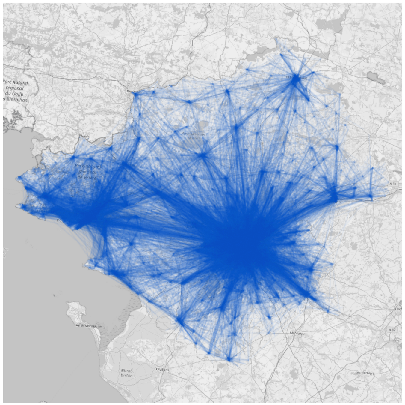
- They allow for a detailed sociodemographic and geographic analysis of patterns, policies and are used in agent-based simulation
- Goal: evaluate spatially and socially eligibility for the 2026 social leasing campaign in France.
- Problem: correctly impute household income information to the synthetic population


0:00 - 9:00
10:00 - 17:30
17:45 - 21:00
22:00 - 0:00


x 60,000,000
A comment on Filosofi
- The Filosofi dataset provided income distributions by household type and / or geographic zone - an integration into eqasim exists
- Decommissioned in 2023, so we need to find a new method!
- Disclaimer: Filosofi 2 exists now, didn't look at it in detail (but only median values seem to be given
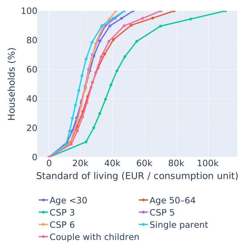
Two alternative data sources
ERFS (2023)
IRCOM (2024)
- Provides the Standard of Living S of households in Metropolitan France
- Link to socio-demographic attributes of a household
- By household type (single M, single F, couple, ...)
- By age group of the reference person* (<30, 30 - 39, ...)
- By socio-professional group (CSP)
- For each uni-dimensional modality (30 - 39, couple, ...) the percentage of households is given (on ten unaligned income brackets)
- Households refer to people living in the same housing unit
- Provides statistics on collected income tax, including the fiscal reference revenue R of households (révenue fiscal de réference; RFR)
- Link to geogaphical zones
- By department
- By municipality (for some with sufficient inhabitants)
- Number of households within a given bracket of R
- Brackets globally aligned
- Households refer to tax households (foyer fiscal)
Two alternative data sources
ERFS (2023)
IRCOM (2024)
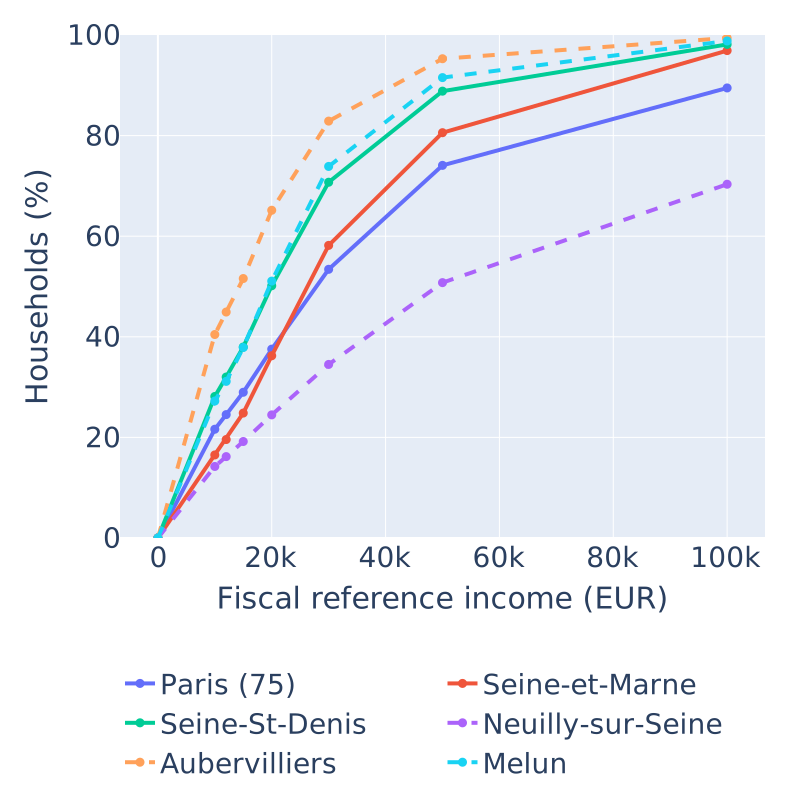
Two alternative data sources
ERFS (2023)
IRCOM (2024)
S = T / U
Standard of living
Disposable household income
Consumption units
After taxes, social benefits, ...
1 for first adult + 0.5 for additional adult + 0.3 per child (<14)
R = f(H) = ?
Reference fiscal income
No direct correspondance to S or H!
Basis for income tax calulation
Census data as a basis
Census (2021)
- Provides weighted household observations across France with a sampling rate of about 30%
- Already integrates a flag for the reference person of a household
- Allows us to count household observations
- with reference person in age group A
- with reference person in CSP C
- with household type H
- inside zone Z
- either Z = M for municipalities
- or Z = D for deaprtments
Census tensor
Census data as a basis
Census (2021)
- Provides weighted household observations across France with a sampling rate of about 30%
- Already integrates a flag for the reference person of a household
- Allows us to count household observations
- with reference person in age group A
- with reference person in CSP C
- with household type H
- inside zone Z
- either Z = M for municipalities
- or Z = D for deaprtments
- with consumption units U
- Need to create finite number of brackets
Census tensor
Standard of living model
Census tensor
Standard of living model
Census tensor
Standard of living tensors
- Agree on aligned S brackets over all distributions
- Resample the provided ERFS distributions
- Then count number of househods in each bracket for given modality
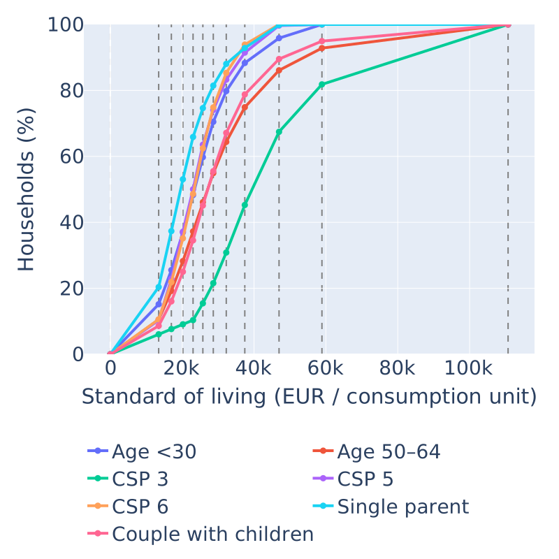
Resampled ERFS
Standard of living model
Census tensor
Standard of living tensors
Standard of living model
s.t.
- Construct a new tensor M that fits
- Census marginal tensor
- ERFS marginals
- Can be solved using Iterative Proportional Fitting!
Standard of living model
Standard of living model
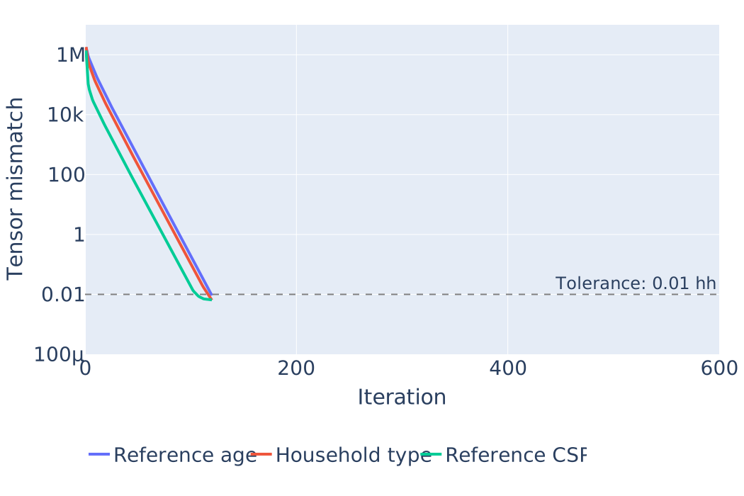
Standard of living model
Standard of living model
- Obtain (A, C, H) for each household in the synthetic population
- Sample from P(S | A, C, H)
Spatialized model
Census tensor
Standard of living tensors
Geographical tensor
Spatialized model
Census tensor
Standard of living tensors
Geographical tensor
Problem 1
S is normalized by consumption units, R is absolute for a household
Problem 2
There is no link between R and S in our model
Spatialized model
Census tensor
Standard of living tensors
Geographical tensor
Problem 1
S is normalized by consumption units, R is absolute for a household
Problem 2
There is no link between R and S in our model
Linking tensor
Spatialized model
Establishing a distribution of T
- Sample N = Large observations of households
- Sample standard of living for each obs.
- Calculate disposable income T for each obs.
- This gives us an empirical approximation of the distribution P(T) in France
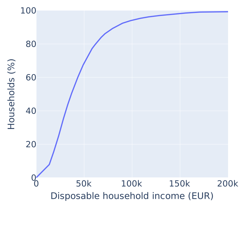
Constructed disposable income
Spatialized model
Establishing a distribution of T
- Sample N = Large observations of households
- Sample standard of living for each obs.
- Calculate disposable income T for each obs.
- This gives us an empirical approximation of the distribution P(T) in France
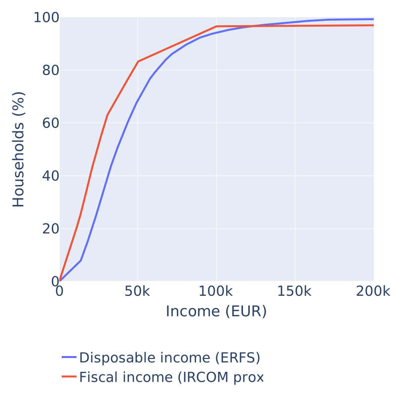
Piecewise-linear approximation of F(R)
- Given the brackets of R and France-wide household counts, we can construct a piecewise-linear distribution F(R)
- Major assumption: A household that is at the kth quantile of F(R) is roughly at the kth quantile of F(T).
Spatialized model
Establishing a distribution of T
- Sample N = Large observations of households
- Sample standard of living for each obs.
- Calculate disposable income T for each obs.
- This gives us an empirical approximation of the distribution P(T) in France
Piecewise-linear approximation of F(R)
- Given the brackets of R and France-wide household counts, we can construct a piecewise-linear distribution F(R)
- Major assumption: A household that is at the kth quantile of F(R) is roughly at the kth quantile of F(T).
- We locate each t on the distribution of R
- Going back to categorical S and R: count how many observations i fall in each combination of (U, S, R):
Spatialized model
Distribution matching
Linking tensor
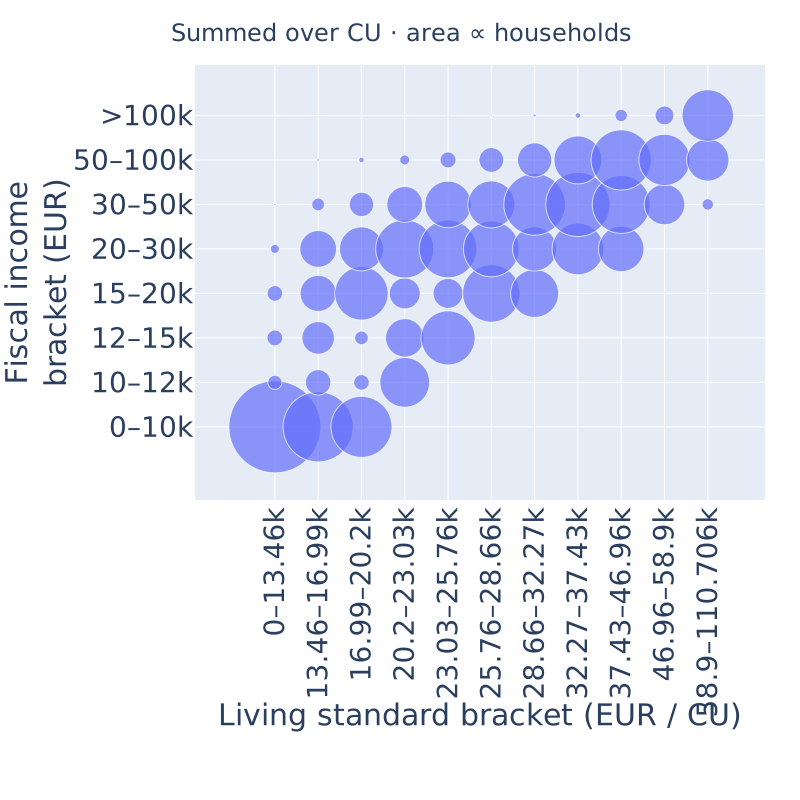
Distribution matching
Linking tensor
(consumption units marginalized out)
Spatialized model
Geographical model
s.t.
- Department version: all departments have information
- Municipality version: substract known municipality (M, R) counts from (D, R) to obtain "unknown" municipality counts, treat them as one group
Spatialized model
- Department version: all departments have information
- Municipality version: substract known municipality (M, R) counts from (D, R) to obtain "unknown" municipality counts, treat them as one group
6 x 7 x 6 x 81 x 96 x 11 x 8 = about 172M cells
6 x 7 x 6 x 81 x 1,944 x 11 x 8 = about 3.5B cells
Running on ~32 GB memory applying sparse matrix calculation
~4h
~24h
Spatialized model
Convergence
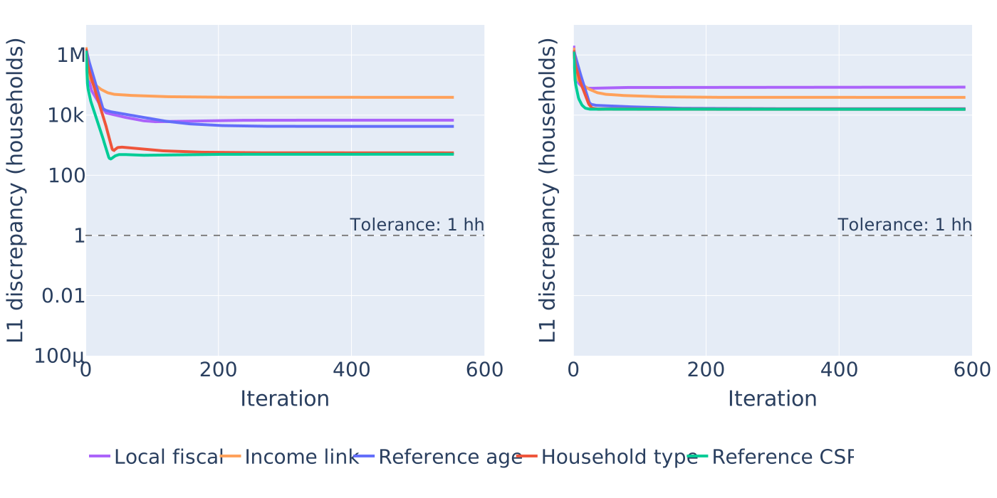
Fitting the geographical model
Spatialized model
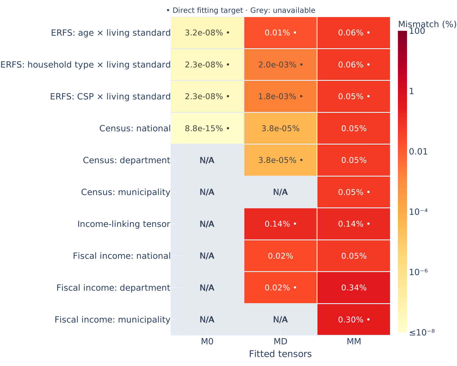
Some first validation results
- Percentage of mismatched observations for each marginal, relative to the stratum size
Spatialized model
Application to a synthetic population
- Create a spatially biased model of S:
- For each household (A, C, H, U, Z) sample
- Calculate disposable income, then r:
(here, S is already spatialized)
Spatialized model
Application to a synthetic population
- Create a spatially biased model of S:
- For each household (A, C, H, U, Z) sample
- Calculate disposable income, then r:
(here, S is already spatialized)
Useful: Fiscal reference income per part
- One part for each adult
- 0.5 parts for the first and second child
- One part for third and more child
Application case
Social leasing eligibility
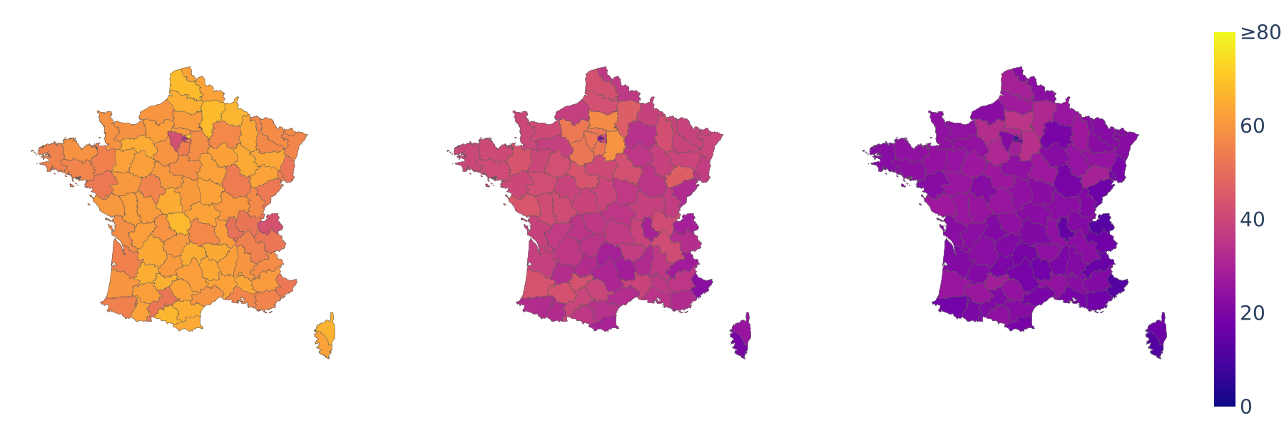
- Commuting distance > 10km
- Obtained from synthetic population's activity chains
- Simplification (here): Euclidean distance!
- Add a distance eligibility to each person
- Fiscal reference income per part <= 16,880 EUR
- Impute income on the synthetic population
- Calculate the RFR par part for each household
- Add an income eligibility flag for each household
- A person is eligible if they are both distance and income eligible!
- We focus on working persons with at least one car in the household!
Application case
Income eligibility
Distance eligibility
Combined
Eligibility [%]
Spatial eligibility analysis
Application case
Social eligibility
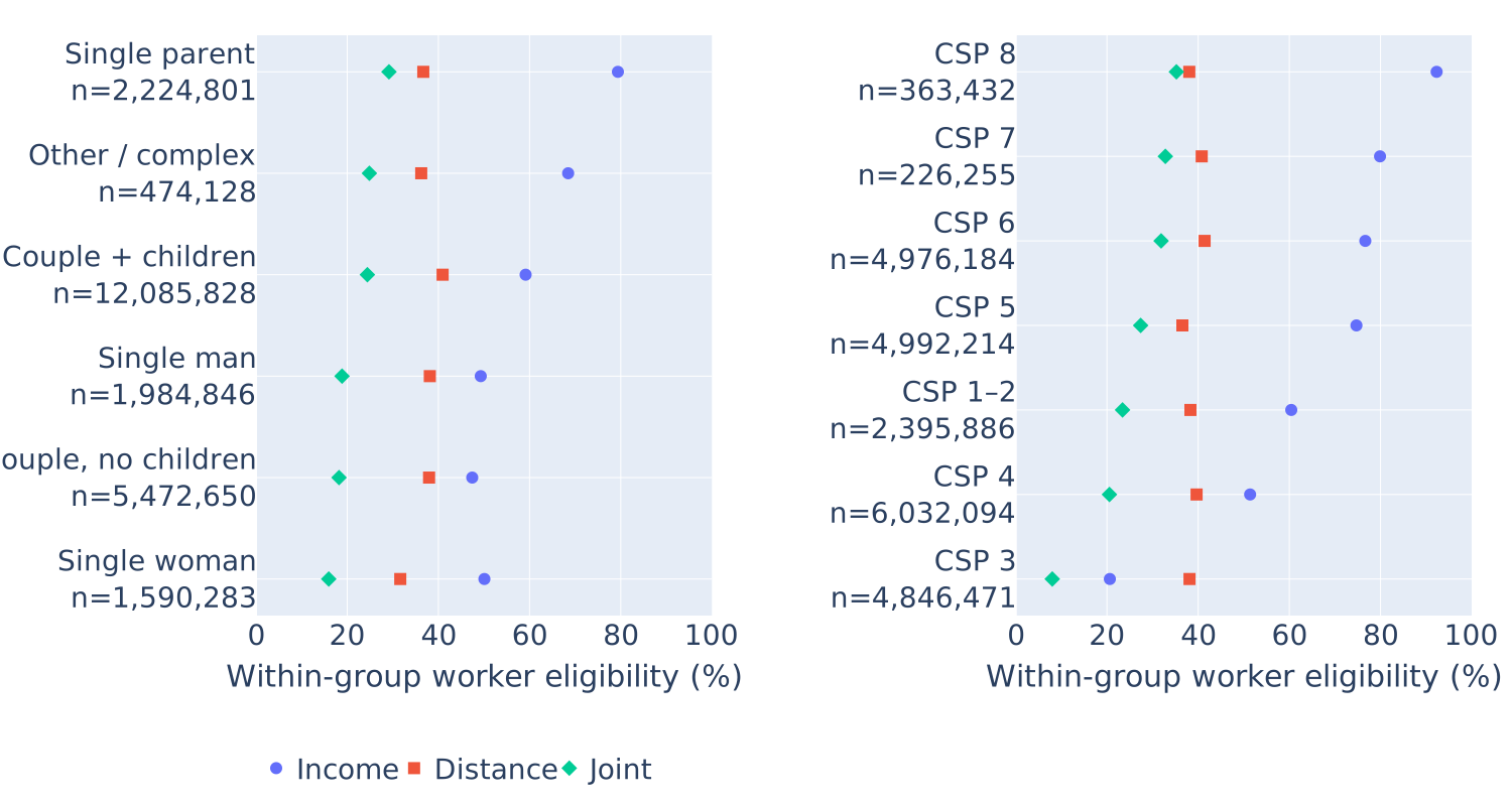
Example: Social eligibility analysis
Application case
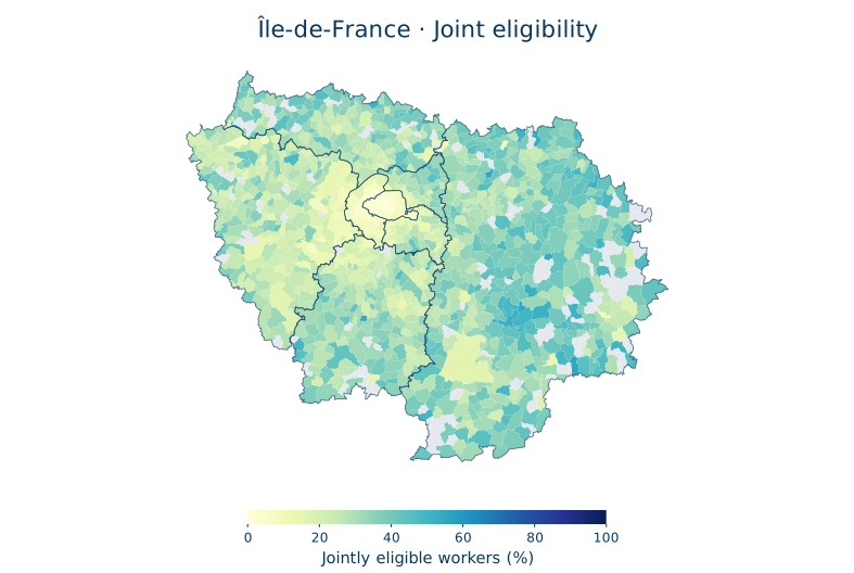
Focus on Île-de-France
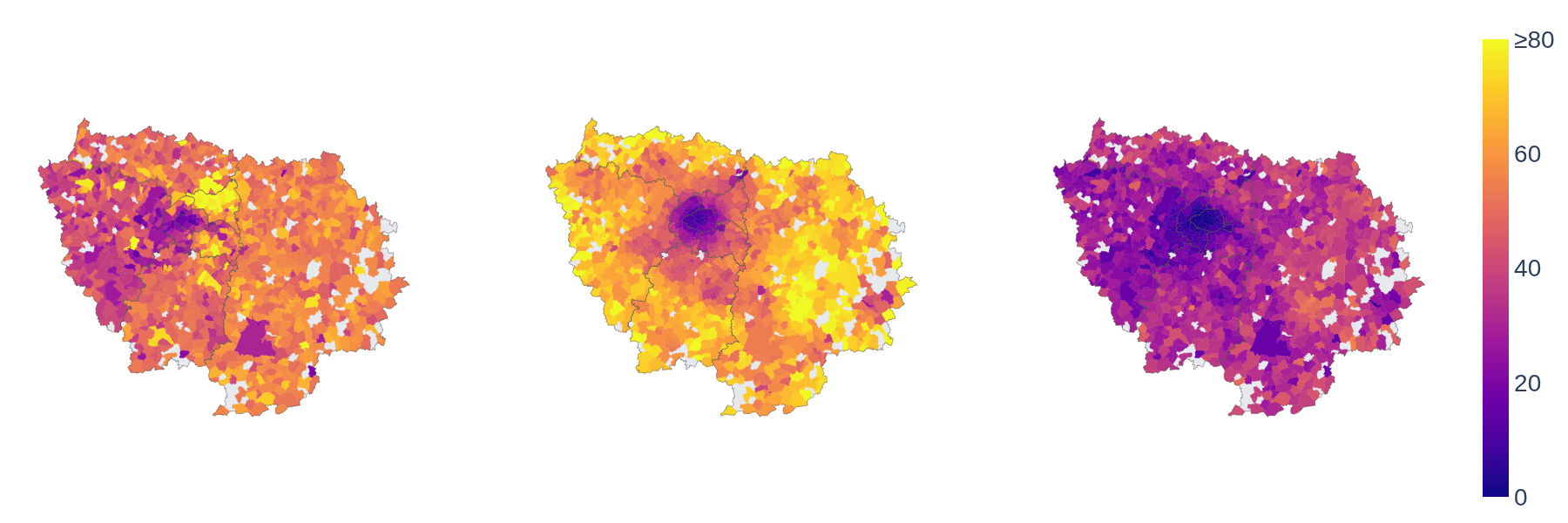
Income eligibility
Distance eligibility
Combined
Eligibility [%]
Application case
Focus on Île-de-France
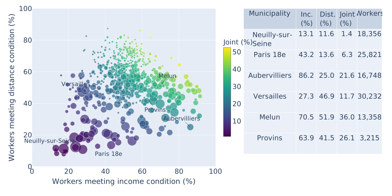
Eligibility [%]
Eligibility [%]
Next steps
Validate our main assumptions
- Quantile-matching of disposable income and fiscal reference income
- Quantile matching between ménages in the census sense and foyers fiscal in tax decalaration sense
Validation with reference data
- Filosofi 2? Household travel surveys?
Technical
- Ensemble runs to test sensitivity over multiple random seeds
- More benchmarking for RAM and computation
Social leasing use case
- Routed distance all across France (osmr)
- Cross with open data on public charging stations: Where is the leasing potential blocked because the infrastructure is not available?
Thank you!
sebastian.horl@irt-systemx.fr
Icons throughout the presentation: https://fontawesome.com
Website
Contact

