Sebastián Ordoñez-Soto
jsordonezs@unal.edu.co
Universidad Nacional de Colombia
Supervisors: Alberto C. dos Reis and Diego Milanés


Dalitz plot analysis of the \(D^{+}\rightarrow K^{-}K^{+}K^{+}\) decay

7th Colombian Meeting on High Energy Physics
December 2, 2022

Contents
- Introduction
- Data samples
- Data selection
- Initial data samples
- Pre-selection
- MVA
- Figures of Merit
- Background model
- Summary
Introduction
- Decays of \(D\) mesons into three final state hadrons are an important tool for studies of low energy QCD.
- These decays proceed dominantly through intermediate resonances, in particular, scalar states which are still poorly understood.
- The scalar states with mass below 1.7 GeV couple to \(\pi\pi\), \(K\pi\) and \(K\bar{K}\) and are produced in decays with a pair of identical particles in the final state, e.g., \(D^{+}\rightarrow K^{-}\pi^{+}\pi^{+}\), \(D^{+}_{(s)}\rightarrow \pi^{-}\pi^{+}\pi^{+}\) and \(D^{+}\rightarrow K^{-}K^{+}K^{+}\).
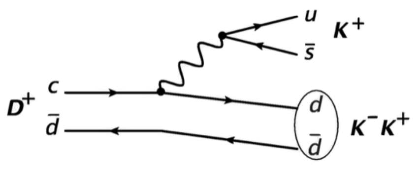
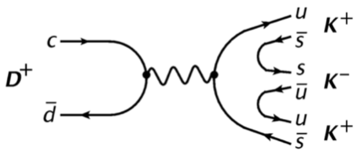
Tree and annhihilation diagrams for the resonant decays of \(D^{+}\rightarrow K^{-}K^{+}K^{+}\) final state
Data and simulation samples
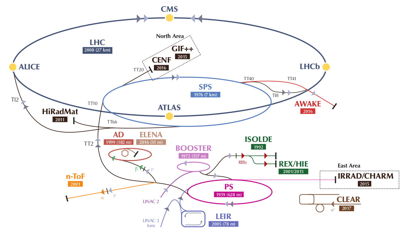
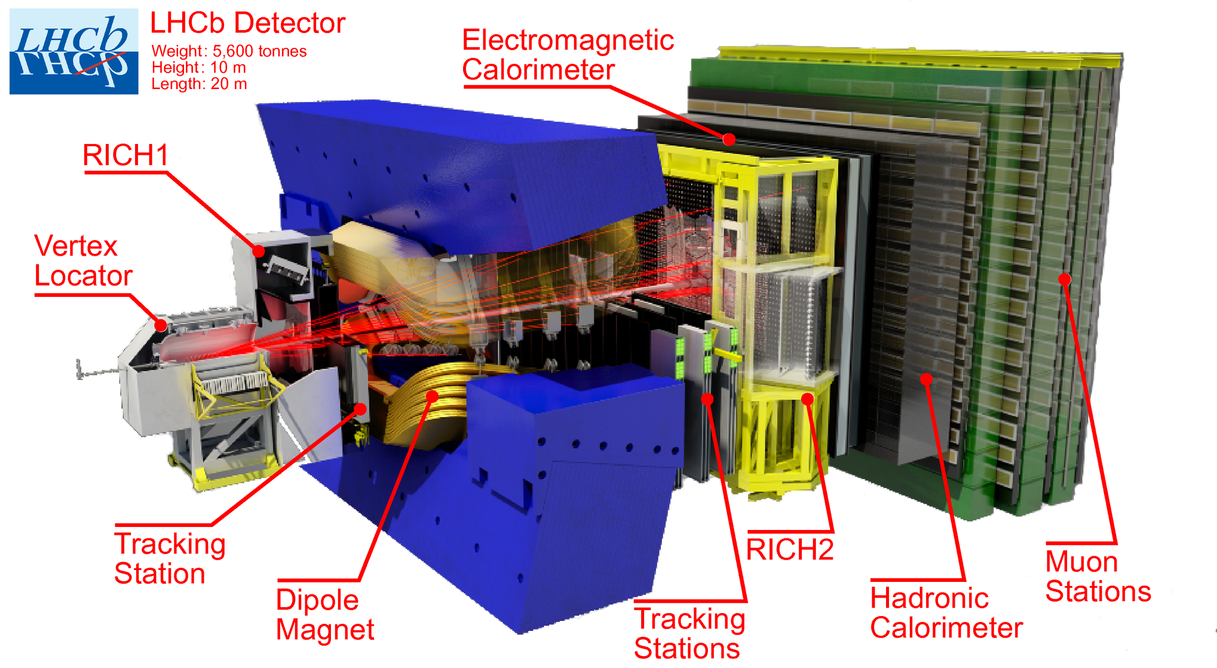
- Data collected in \(pp\) collisions at \(\sqrt{s} = 13\) TeV by LHCb in the Run 2 (2016-2018), which in total corresponds to 5.6 fb\(^{-1}\) of integrated luminosity.
-
Exclusive HLT2 Turbo lines Hlt2CharmHadDpToKmKpKp select the \(D^{+}\rightarrow K^{-}K^{+}K^{+}\) candidates.
-
- Monte Carlo (MC) simulated data is available. Similar configurations for each year but with different trigger settings.
Data selection: Initial data samples
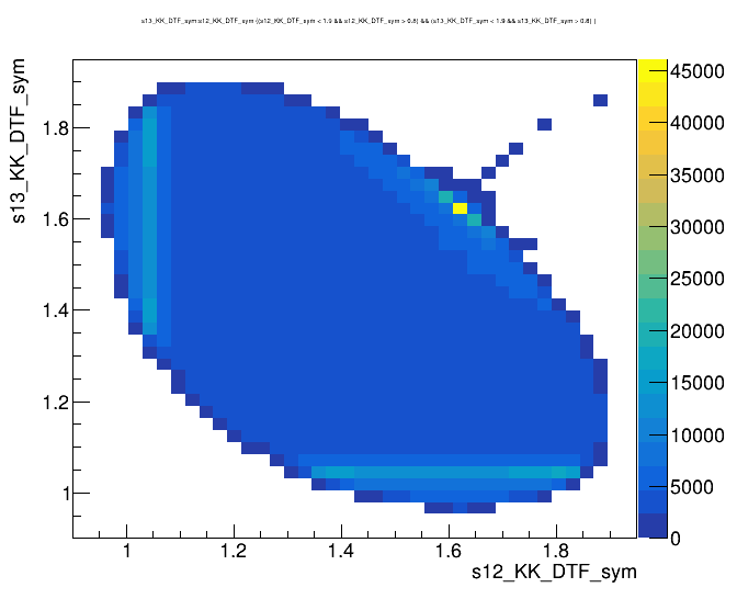
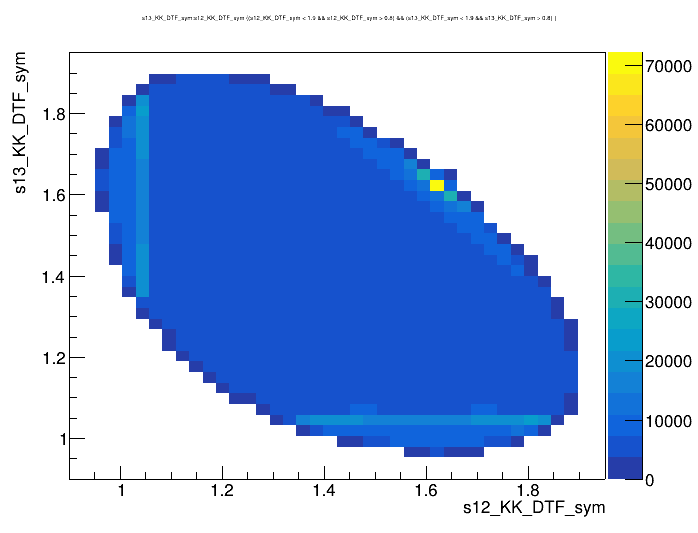
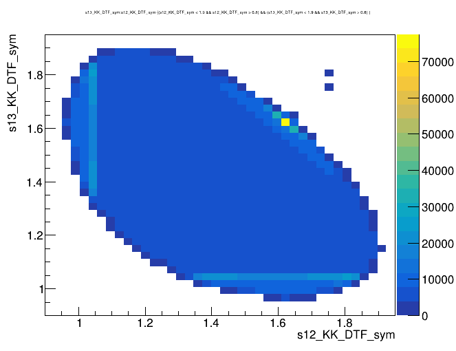
Dalitz plot of the \(D^{+}\) candidates
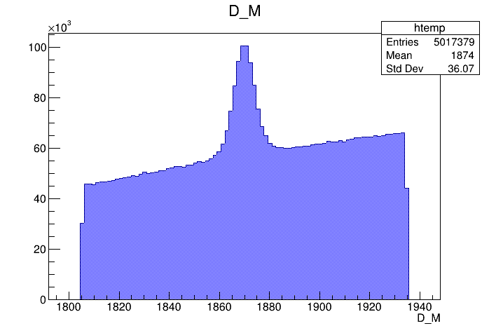
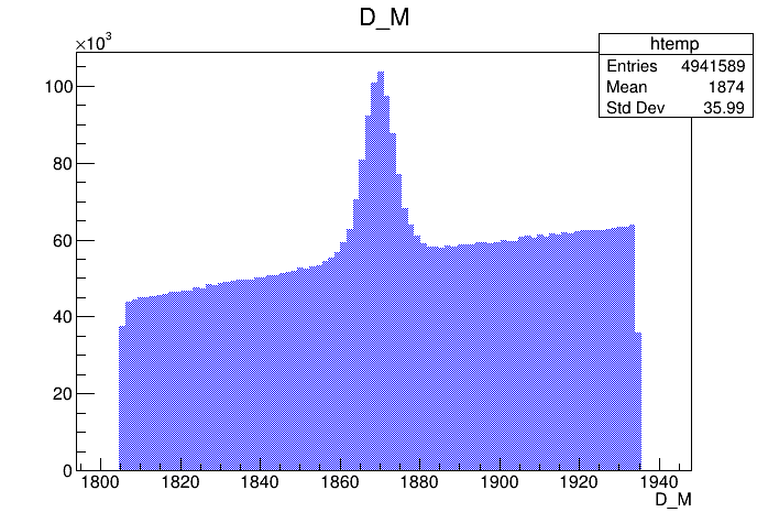
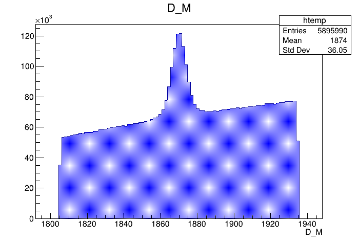
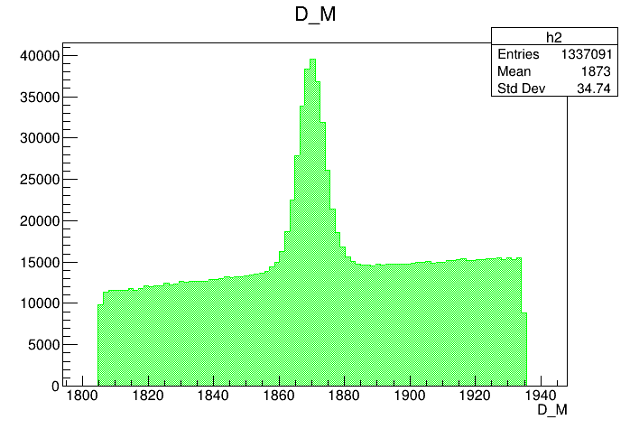
Invariant mass distribution (IMD) of the \(D^{+}\) candidates
\(s_{12}\) (GeV)
\(s_{13}\) (GeV)
\(m_{K^{-}K^{+}K^{+}}\) (MeV)
\(D^{+}\)
Left sideband
Right sideband
\(1869.66 \pm0.05\) MeV
Signal region
Events / MeV
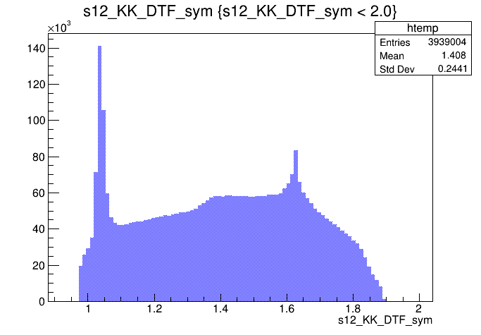
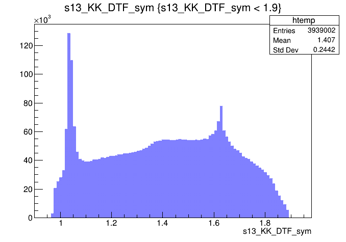
- Mass distributions and Dalitz plots for the 2016-Down data before the pre-selection.
- The data samples have high levels of background: combinatorial and specific backgrounds
- Notation: \(s_{12} = m^{2}(K_{1} ^{-}K_{2}^{+})\) and \(s_{13} = m^{2}(K_{1}^{+}K_{3}^{+})\).

2016-Down
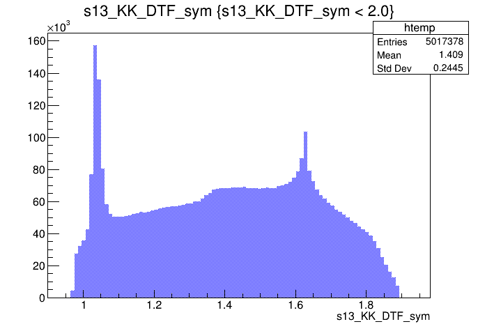
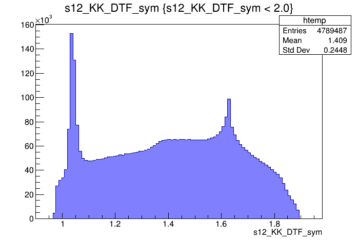
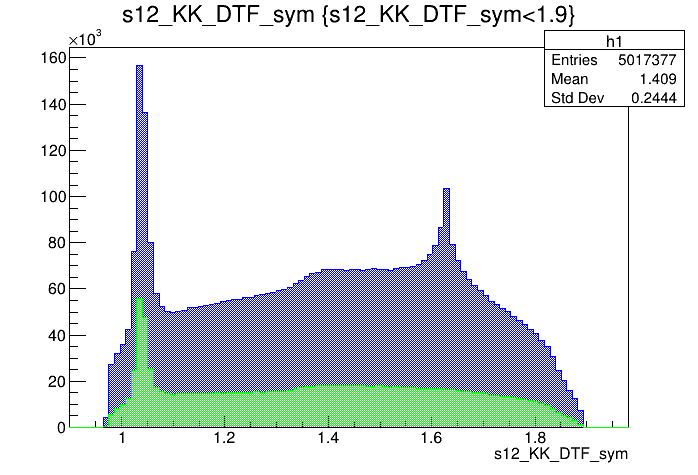
\(s_{12}\) projection of the Dalitz plot
\(s_{13}\) projection of the Dalitz plot
\(s_{12}\) (GeV)
\(s_{13}\) (GeV)
Clone tracks
Clone tracks
Events / GeV\(^{2}\)
Events / GeV\(^{2}\)
Data selection: Initial data samples
2016-Up
Dalitz plot of the \(D^{+}\) candidates
Invariant mass distribution of the \(D^{+}\) candidates
\(m_{K^{-}K^{+}K^{+}}\) (MeV)
\(s_{12}\) (GeV)
\(s_{13}\) (GeV)
Events / MeV
Data selection: Initial data samples
\(s_{12}\) projection of the Dalitz plot
\(s_{13}\) projection of the Dalitz plot
2016-Up
\(s_{12}\) (GeV)
\(s_{13}\) (GeV)
Events / GeV\(^{2}\)
Events / GeV\(^{2}\)
Data selection: Initial data samples
2017-Down

Dalitz plot of the \(D^{+}\) candidates
Invariant mass distribution of the \(D^{+}\) candidates
\(m_{K^{-}K^{+}K^{+}}\) (MeV)
\(s_{12}\) (GeV)
\(s_{13}\) (GeV)
Events / MeV
Data selection: Initial data samples
2017-Down


\(s_{12}\) projection of the Dalitz plot
\(s_{13}\) projection of the Dalitz plot
\(s_{13}\) (GeV)
\(s_{12}\) (GeV)
Events / GeV\(^{2}\)
Events / GeV\(^{2}\)
Data selection: Initial data samples
2017-Up

Dalitz plot of the \(D^{+}\) candidates
Invariant mass distribution of the \(D^{+}\) candidates
\(m_{K^{-}K^{+}K^{+}}\) (MeV)
\(s_{12}\) (GeV)
\(s_{13}\) (GeV)
Events / MeV
Data selection: Initial data samples
2017-Up

\(s_{12}\) projection of the Dalitz plot
\(s_{13}\) projection of the Dalitz plot
\(s_{12}\) (GeV)
\(s_{13}\) (GeV)
Events / GeV\(^{2}\)
Events / GeV\(^{2}\)
Data selection: Initial data samples
2018-Down

Dalitz plot of the \(D^{+}\) candidates
Invariant mass distribution of the \(D^{+}\) candidates
\(m_{K^{-}K^{+}K^{+}}\) (MeV)
\(s_{12}\) (GeV)
\(s_{13}\) (GeV)
Events / MeV
Data selection: Initial data samples
2018-Down


\(s_{12}\) projection of the Dalitz plot
\(s_{13}\) projection of the Dalitz plot
\(s_{12}\) (GeV)
\(s_{13}\) (GeV)
Events / GeV\(^{2}\)
Events / GeV\(^{2}\)
Data selection: Initial data samples
2018-Up
Dalitz plot of the \(D^{+}\) candidates
Invariant mass distribution of the \(D^{+}\) candidates
\(m_{K^{-}K^{+}K^{+}}\) (MeV)
\(s_{12}\) (GeV)
\(s_{13}\) (GeV)
Candidates / MeV
Data selection: Initial data samples
2018-Up

\(s_{12}\) projection of the Dalitz plot
\(s_{13}\) projection of the Dalitz plot
\(s_{12}\) (GeV)
\(s_{13}\) (GeV)
Events / GeV\(^{2}\)
Events / GeV\(^{2}\)
Data selection: Initial data samples
\(s_{12}\) (GeV)
\(s_{13}\) (GeV)
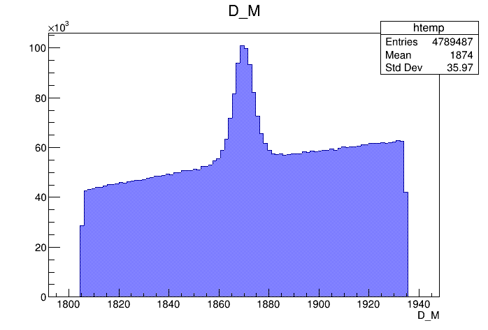
\(m_{K^{-}K^{+}K^{+}}\) (MeV)
Dalitz plot of the \(D^{+}\) pre-selected candidates
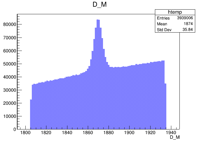
Mass distribution of the \(D^{+}\) pre-selected candidates
Events / MeV
\(D^{+}\)
Data selection: Pre-selection
- Mass distributions and Dalitz plots for the 2016-Down data after the pre-selection.
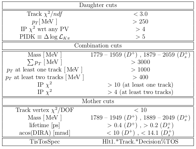
- There is charm background in the \(K^{-}K^{+}K^{+}\) mass spectrum due to misidentification (mis-ID), e.g., \(D^{+}_{s} \rightarrow K^{-}K^{+}\pi^{+}\pi^{0}\), \(D^{+} \rightarrow K^{-}K^{+}\pi^{+}\pi^{0}\), \(\Lambda_{c}^{+}\rightarrow K^{-}K^{+}p\) and \(\Lambda_{c}^{+}\rightarrow K^{-}\pi^{+}p\).
- Particle identification (PID) cuts are used to control the peaking background: probNNk\(_{1,2,3}\) > 0.6 cut
\(m_{K^{-}K^{+}K^{+}}\) (MeV)
\(s_{12}\) (GeV)
\(s_{12}\) projection of the Dalitz plot
\(s_{13}\) projection of the Dalitz plot
Events / MeV
Events / MeV
\(D^{+}\)
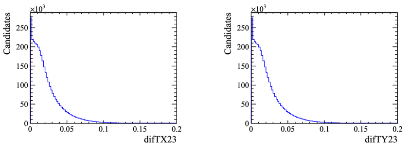
Data selection: Pre-selection
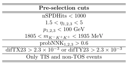
- The next specific contribution eliminated was that of cloned tracks of the \(K^{+}\) daughters.
- To remove these events, the following two slope difference variables were used:
\(\phi\) (1020)
Data selection: Multivariate Analysis
2016-Down (Fold 1)
Sidebands from data
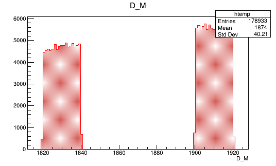
Input data for training
\(m_{K^{-}K^{+}K^{+}}\) (MeV)
\(m_{K^{-}K^{+}K^{+}}\) (MeV)
Invariant mass distribution of the \(D^{+}\) simulated candidates
Events / MeV
Events / MeV
\(D^{+}_{MC}\)
2016-Down (Fold 1)
- A MultiVariate Analysis (MVA) is used to reduce the combinatorial contribution to the \(D^{+}\rightarrow K^{-}K^{+}K^{+}\).
- The three main stages of the MVA are: training, testing and application.
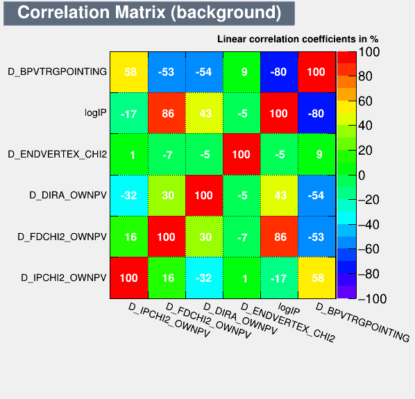
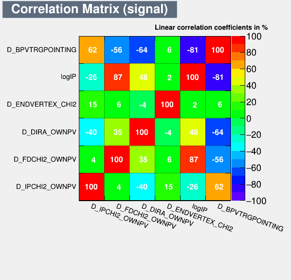
- For the training, a reweighted MC sample is used as signal and data sidebands are used as background.
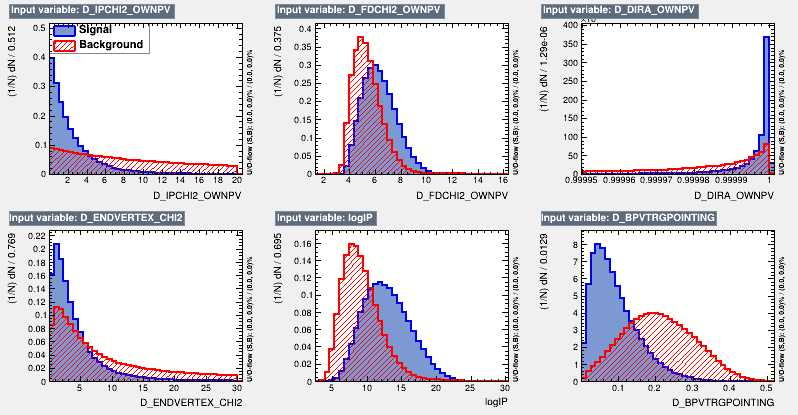
- These variables are chosen for the MVA training because of their discriminating power.
Data selection: Multivariate Analysis
MVA training results
- 1M signal events and 900k background events were used for the training of the BDTG classifier.
MVA testing results
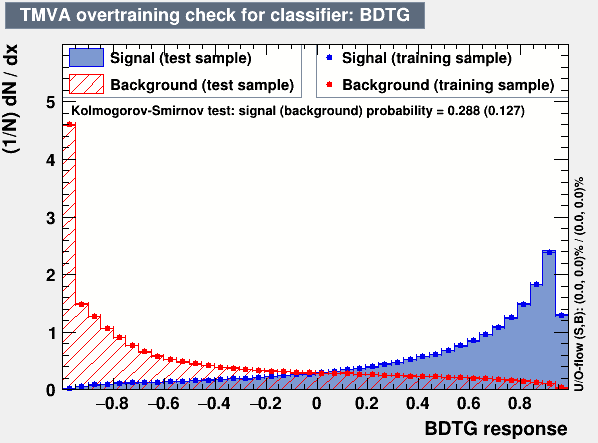
Overtraining check
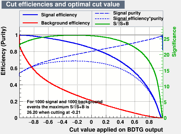
Figures of merit
Data selection: Multivariate Analysis
- 100k signal events and 100k background events were used for the testing of the BDTG classifier.
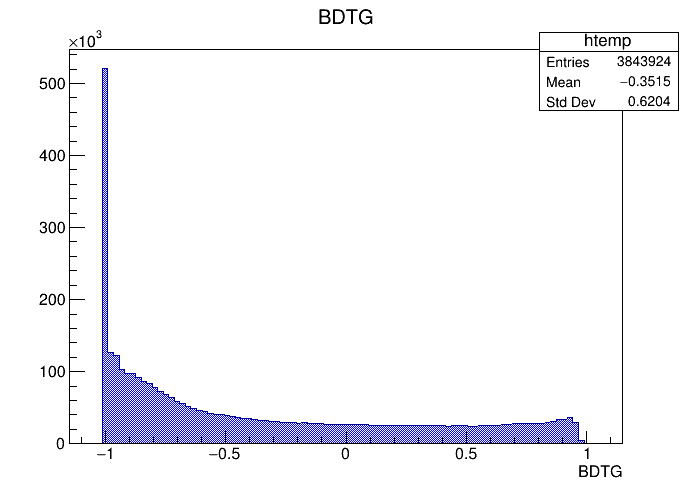
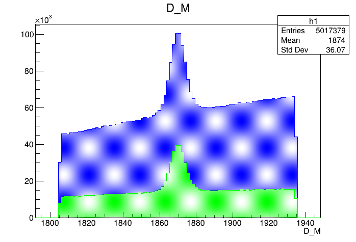
BDTG application on Data
Events
Events
MVA application results
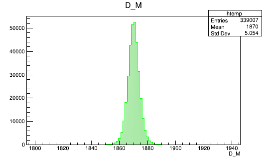
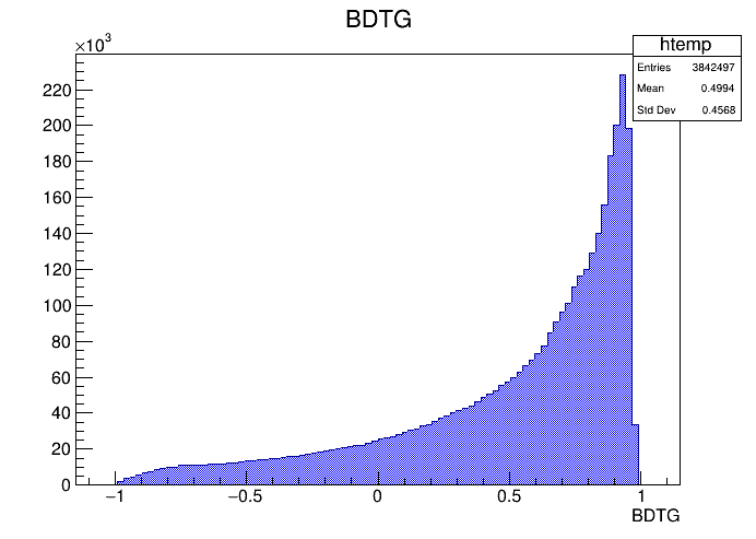
BDTG application on MC
Fold 2
Fold 2
- The last step of the MVA is to apply the resulting BDTG classifier in non-labeled data
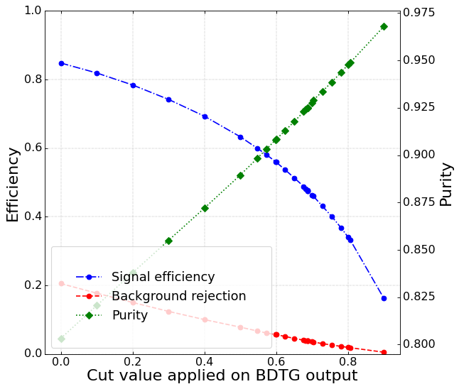
- A tighter cut on the BDTG_val variable give us a higher signal purity with a loss in signal efficiency.
Data selection: Multivariate Analysis
Data selection: Figures of merit
Signal efficiency and purity
- In Dalitz plot analysis high purity samples are required.
- Purity is defined as:
- Signal efficicency is calculated as:
Fold 2
Data analysis: Figures of merit
Fits after BDTG cut
\(D^{+}\)
\(D^{+}\)
\(m_{K^{-}K^{+}K^{+}}\) (MeV)
Candidates / MeV
-
If the cut BDTG_val > 0.68 is applied, a signal purity of 92.5% and a signal efficiency of 48% are reached.
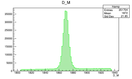
IMD of the final \(D^{+}\) candidates
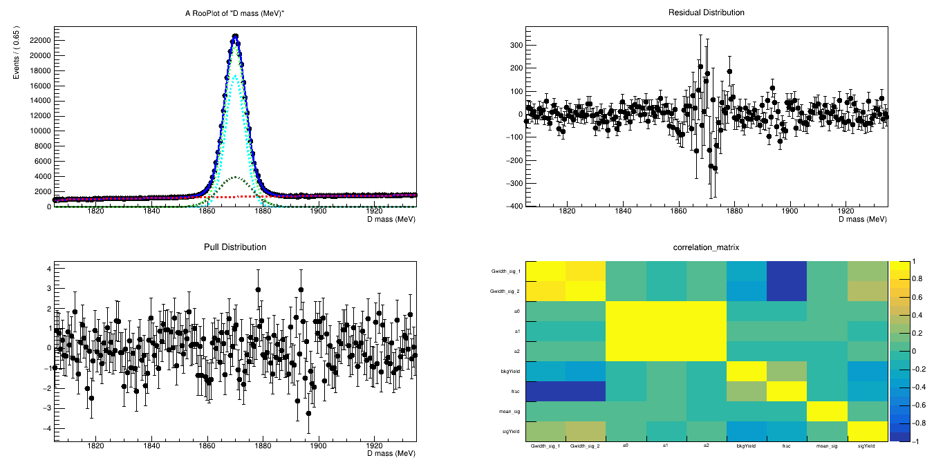
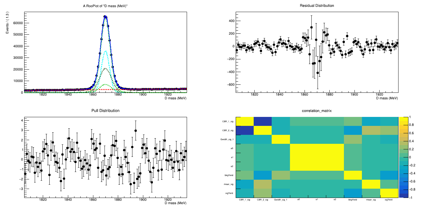
Fit to the final mass distribution
Fold 2
Fold 2
Data selection: Final sample
\(m_{K^{-}K^{+}K^{+}}\) (MeV)
\(m_{K^{-}K^{+}K^{+}}\) (MeV)
Candidates / MeV
Candidates / (1.3 MeV)
\(D^{+}\)
\(D^{+}\)
- The final sample contains 505 thousand candidates in the signal region, of which (92.52 \(\pm\) 0.07 )% correspond to signal.
IMD of the final \(D^{+}\) candidates
Fit to the final mass distribution
- This is 4.55 times the statistics of the same analysis with the Run 1.
Data selection: Final sample
Candidates / GeV\(^{2}\)
\(s_{12}\) (GeV)
\(s_{12}\) (GeV)
\(s_{13}\) (GeV)
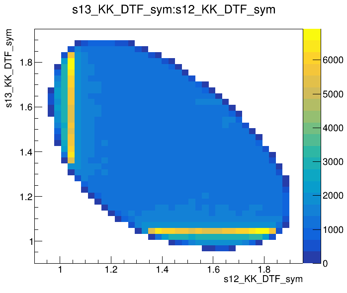
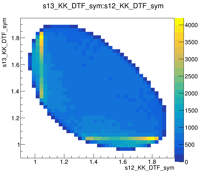
Dalitz plot of the \(D^{+}\) candidates
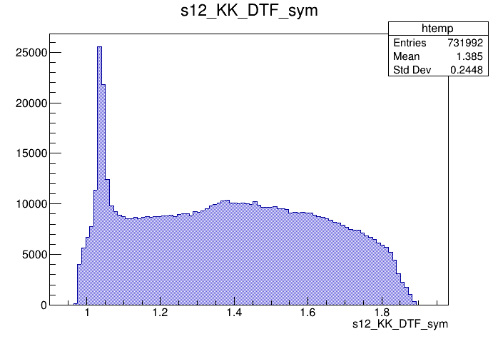
\(s_{12}\) projection of the Dalitz plot
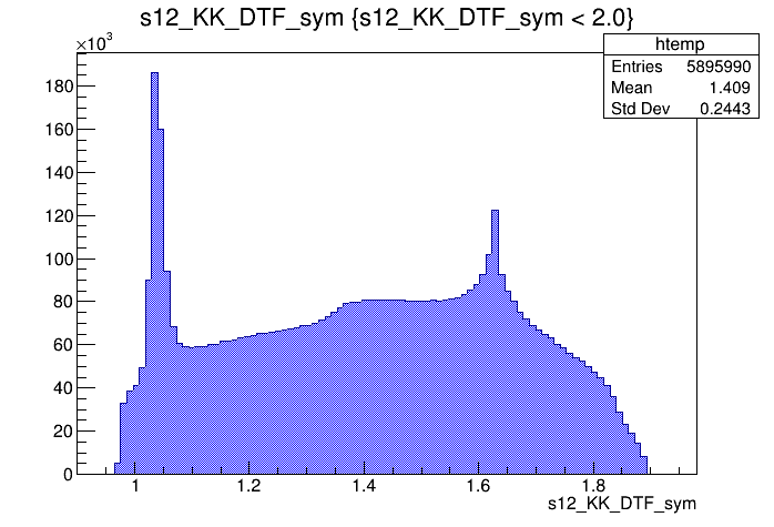
- Dalitz plot and one of its projections for events in the full \(K^{-}K^{+}K^{+}\) spectrum
\(\phi\) (1020)
Data selection: Final sample

\(m_{K^{-}K^{+}K^{+}}\) (MeV)
\(m_{K^{-}K^{+}K^{+}}\) (MeV)
Events / MeV
Events / MeV
\(D^{+}\)
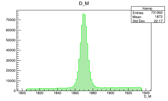
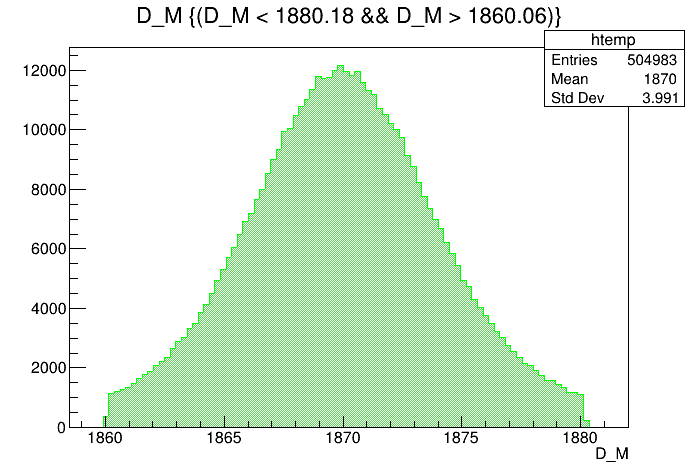
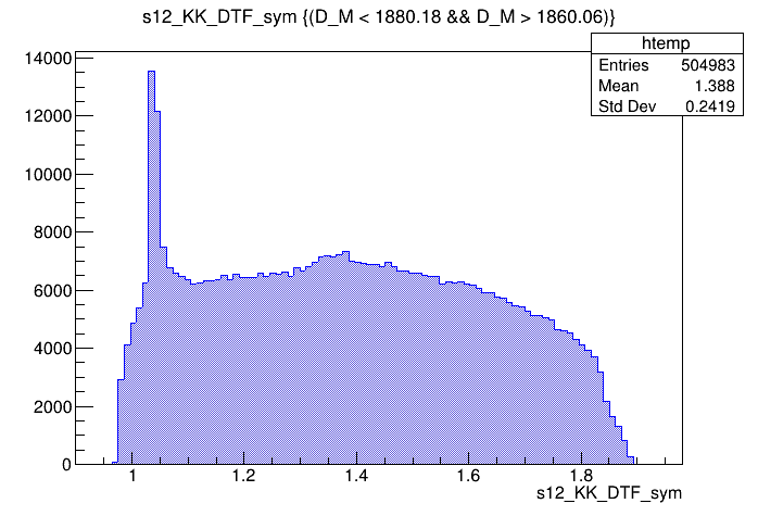
IMD of the final \(D^{+}\) candidates in the signal region
Sidebands of the final data sample
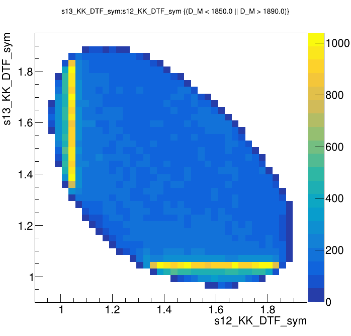
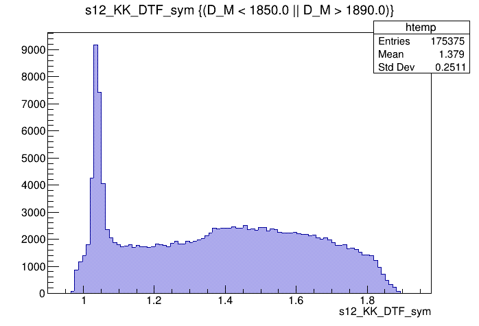
- Let us consider separately the signal region and the sidebands.
Data selection: Final sample
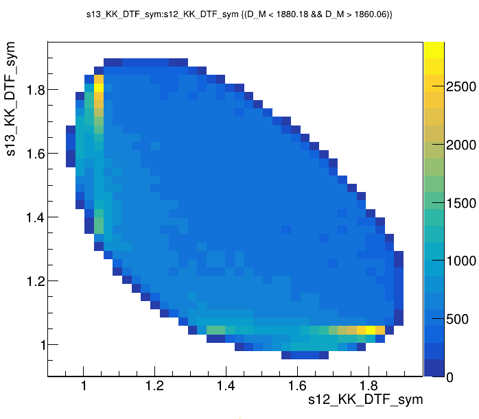
Candidates / GeV\(^{2}\)
\(s_{12}\) (GeV)
\(s_{12}\) (GeV)
\(s_{13}\) (GeV)
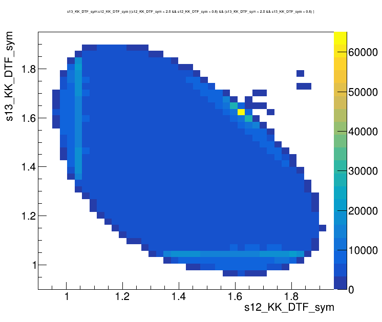
Dalitz plot of the \(D^{+}\) candidates in the signal region
\(s_{12}\) projection of the Dalitz plot from the signal region
Signal region
\(\phi\) (1020)
Data selection: Final sample
Candidates / GeV\(^{2}\)
\(s_{12}\) (GeV)
\(s_{12}\) (GeV)
\(s_{13}\) (GeV)
Dalitz plot of the sidebands events
\(s_{12}\) projection of the Dalitz plot from the sidebands
Sidebands
\(\phi\) (1020)
Background Model
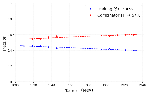
- Work in progress: Study the composition of the remaining background.
- Fits to the Dalitz projections are performed (slices of 9 MeV) and yields for the peaking and combinatorial background are obtained.
Summary
Thank you!
- The pre-selection of the \(D^{+}\rightarrow K^{-}K^{+}K^{+}\)candidates was successfully performed, removing most of the charm background and cloned tracks.
- A Multivariate Analysis was carried out in order to reject the remaining combinatorial background in the \(D^{+}\rightarrow K^{-}K^{+}K^{+}\) mass spectrum.
- Different figures of merit were estimated aiming to find the optimal cut in the resulting MVA classifier output.
- A final sample with 505 thousand \(D^{+}\rightarrow K^{-}K^{+}K^{+}\) candidates and with a purity of (92.52 \(\pm\) 0.07) % was obtained.
Data and simulation samples
HLT2 selection criteria
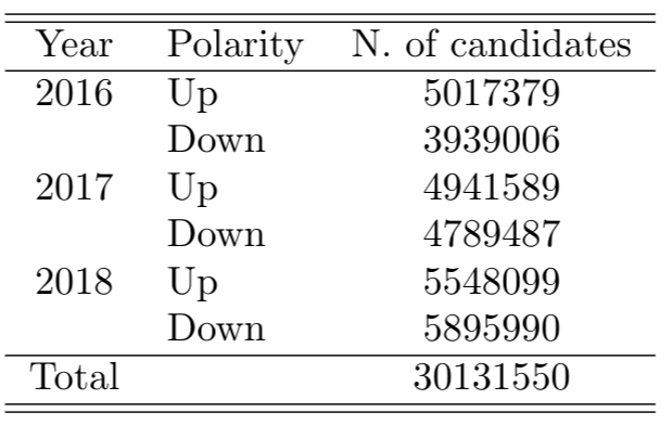
Data selection: Initial data sample
Number of candidates before pre-selection
Data selection: Pre-selection
Summary of pre-selection cuts
Data selection: Pre-selection
Slope difference variables
Data selection: Multivariate Analysis
MVA training results