Contact Sampling for
Contact Rich Manipulation
28 April 2023
By Shao Yuan Chew Chia
Joint work with: Terry Suh, Pang Tao, Sizhe Li
Contact Sampling Problem
Given a goal state \(x_g\) and current state \(x\) of the object,
how should you position the robot \(q\) to best reach \(x_g\),
through subsequent commands \(u\)
\(x_g\)
\(x\)
\(q\)
\(u\)
Why this problem?
Address the discrete question of where/how to make contact
\(x_g\)
\(x\)
\(q_{1}\)
\(q_{2}\)
Why this problem?
Address the discrete question of where/how to make contact
\(x_g\)
\(x\)
\(q_{1}\)
\(q_{2}\)
General Problem Area
Motion planning for high dimensional contact-rich manipulation
| Classes of Methods | Trajectory Optimization | Sampling based motion planning | Learning based methods |
|---|---|---|---|
| Examples | Continuous trajectory optimization |
Rapidly exploring Random Tree (RRT) | Reinforcement Learning, Behavior cloning |
| How contact sampling can help | Provide good initial guesses | Increase state space coverage of "extend" step | Improve sample efficiency |
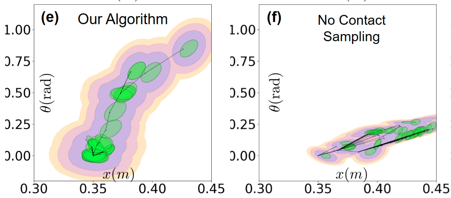
Improving Trajectory Optimization
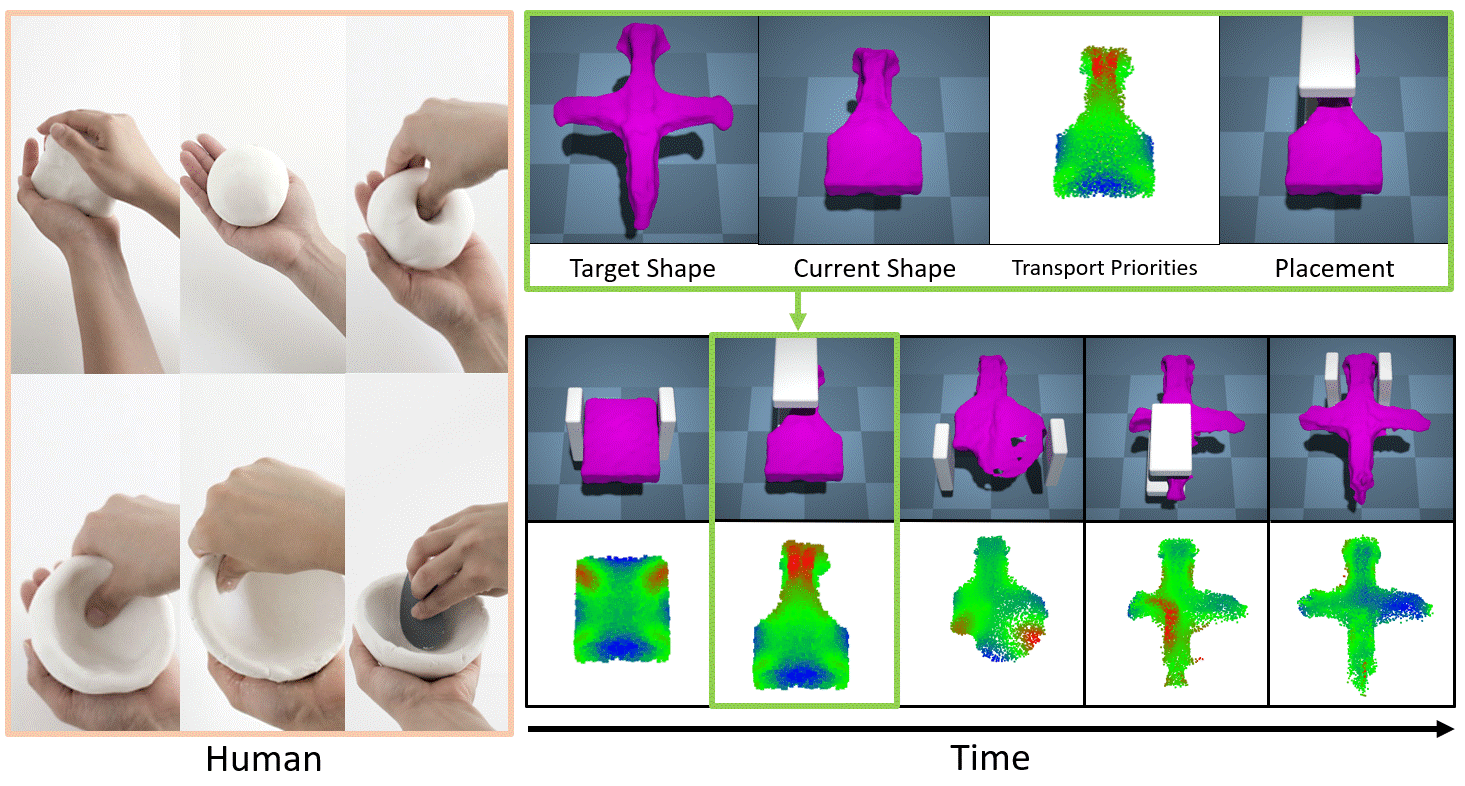
Uses optimal transport to define a heuristic for which particles need to move the most
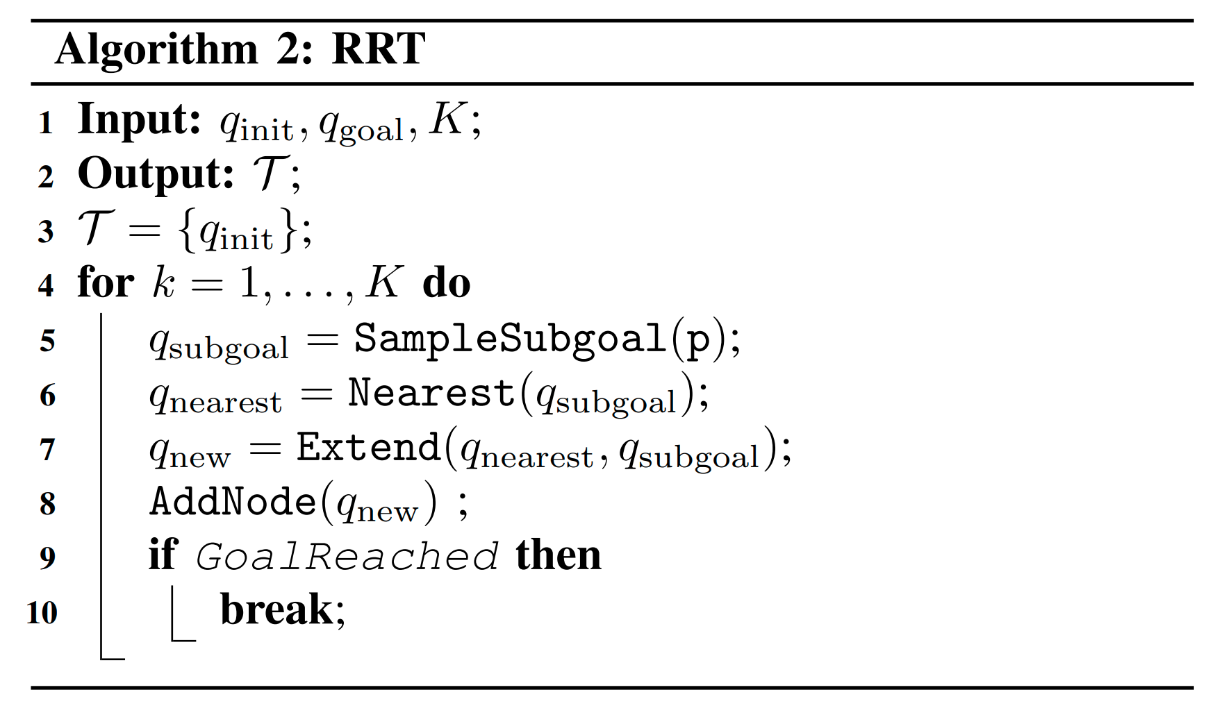
Improving RRT
Contact Sampling Problem
Given a goal state \(x_g\) and current state \(x\) of the object,
how should you position the robot \(q\) to best reach \(x_g\),
through subsequent commands \(u\)
\(x_g\)
\(x\)
\(q\)
\(u\)
Contact Sampling Problem
Given a goal state \(x_g\) and current state \(x\) of the object,
how should you position the robot \(q\) to best reach \(x_g\),
through subsequent commands \(u\)
\(x_g\)
\(x\)
\(q\)
\(u\)
Long horizon question
Modified Problem
Given a goal state \(x_g\) and current state \(x\) of the object,
find the robot position \(q\), that would in one subsequent command \(u\), minimize the object's distance to the goal,
\(x_g\)
\(x\)
\(q\)
\(u\)
Assumptions
-
Discrete time
-
Quasistatic dynamics
-
Absolute position commands
Solution Sketch
Input: \(x\), \(x_g\)
Output: \(N\) best \(q\)'s
- Sample \(M\) initial admissible positions of the robot \(q_0\)
- Rejection sample via collision checker
- Uniform distribution over workspace
- Do gradient descent to evolve the initial positions
- At each step, project \(q\) back into admissible set
- Return \(N\) best \(q\)'s
Key Challenge
contact dynamics lead to the cost landscape being flat
Solution 1:
Randomized Smoothing of the cost
Cost landscape: Randomized Smoothing (Warm up 1)
- [x,y,theta]
- x_init
[0,0,0] (Blue) - x_goal
[2,0,0] (Green)
- x_init
[0,0,0]
(Blue) - x_goal
[-1.5,-1.5,1] (Green)
Cost landscape: Randomized Smoothing (Warm up 2)
Cost landscape: Randomized Smoothing (Distance from Goal)
\(x_g\) = [0.3, 0, 0]
\(x_g\) = [2, 0, 0]
Cost landscape: Randomized Smoothing (Action Standard Deviation, Goal Near)
std = 0.01
std = 0.1
Cost landscape: Randomized Smoothing (Action Standard Deviation, Goal Far)
std = 0.01
std = 0.1
Cost landscape: Randomized Smoothing (Action Standard Deviation Animations)
std = [0.01 , ... , 1]
Cost landscape: Randomized Smoothing
Sample Aggregation Function
Min
Mean
Max
Non-Physical Behavior of Anitescu Convex Relaxation
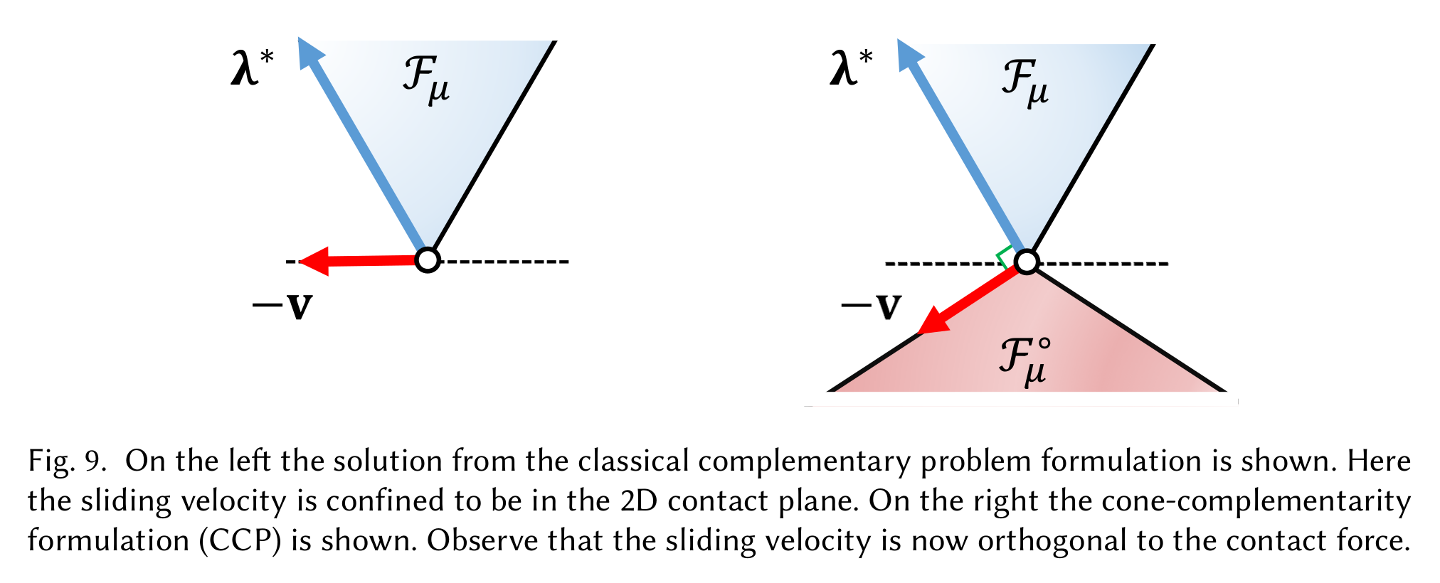
Andrews, S., Erleben, K., & Ferguson, Z. (2022). Contact and friction simulation for computer graphics. In ACM SIGGRAPH 2022 Courses (pp. 1-172).
Non-Physical Behavior of Anitescu Convex Relaxation
Effect on Cost Landcape (std = 0.5)
Incremental steps = 10
Incremental steps = 5
Incremental steps = 1
Non-Physical Behavior of Anitescu Convex Relaxation
Effect on Cost Landcape (std = 0.1)
Incremental steps = 10
Incremental steps = 5
Incremental steps = 1
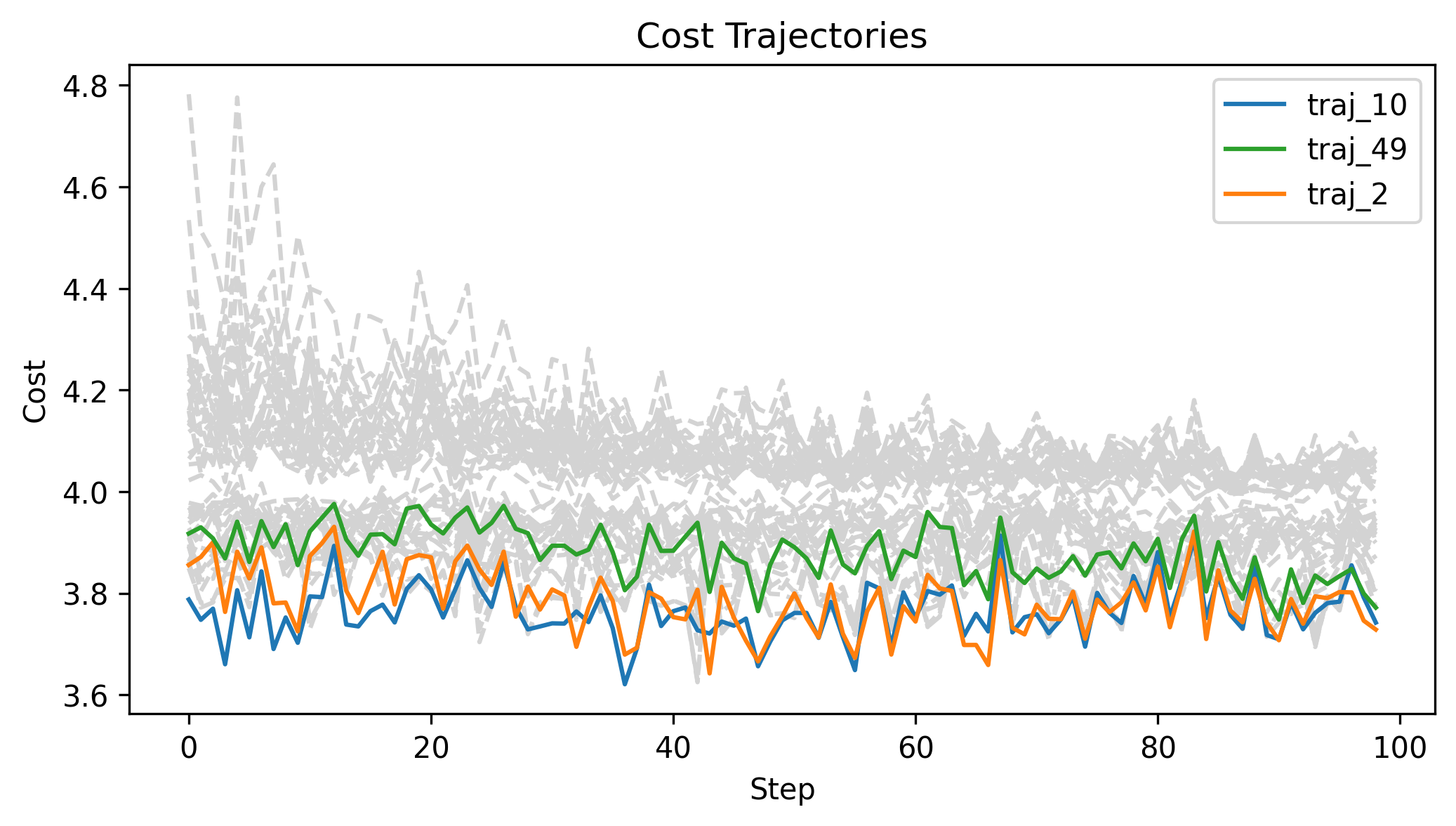
Zeroth Order Batch Gradient
Randomized Smoothing of
cost
Gradient Computation
We want to solve
To use zeroth-order methods, we can instead choose a surrogate objective
Gradient Computation
where
which has the unbiased estimator of the sample mean, i.e.
Gradient Computation
Thus the natural estimator of the gradient is
Zeroth Order Batch Gradient
\(x_g\) = [2,0,0], q_std = 0.1, u_std = 0.1, h=0.01
Zeroth Order Batch Gradient
\(x_g\) = [2,0,0], q_std = 0.1, u_std = 0.1, h=0.01

Zeroth Order Batch Gradient
\(x_g\) = [-1.5,-1.5,1], q_std = 0.1, u_std = 0.1, h=0.01
Zeroth Order Batch Gradient
\(x_g\) = [-1.5,-1.5,1], q_std = 0.1, u_std = 0.1, h=0.01

Zeroth Order Batch Gradient
\(x_g\) = [-1.5,-1.5,1], q_std = 0.1, u_std = 0.1, h=0.01
Zeroth Order Batch Gradient
\(x_g\) = [2,0,0], q_std = 0.1, h=0.01
u_std = 0.1
u_std = 0.3
u_std = 0.5
Zeroth Order Batch Gradient
\(x_g\) = [2,0,0], u_std = 0.3, h=0.01
q_std = 0.05
q_std = 0.1
q_std = 0.3
Zeroth Order Batch Gradient
\(x_g\) = [2,0,0], u_std = 0.3, h=0.05
q_std = 0.05
q_std = 0.1
q_std = 0.3
Solution 2:
Analytic Smoothing of
Contact Dynamics
Cost Landscape: Analytic Smoothing of Contact Dynamics
\(x_g\) = [2,0,0]
Log barrier weight = 1000
(0.001N at 1m)
Log barrier weight = 100
(0.01N at 1m)
Log barrier weight = 10
(0.1N at 1m)
Cost Landscape: Analytic Smoothing of Contact Dynamics
\(x_g\) = [0.3,0,0]
Log barrier weight = 1000
(0.001N at 1m)
Log barrier weight = 100
(0.01N at 1m)
Log barrier weight = 10
(0.1N at 1m)
Cost Landscape: Analytic Smoothing of Contact Dynamics
\(x_g\) = [-1.5,-1.5,1]
Log barrier weight = 1000
(0.001N at 1m)
Log barrier weight = 100
(0.01N at 1m)
Log barrier weight = 10
(0.1N at 1m)
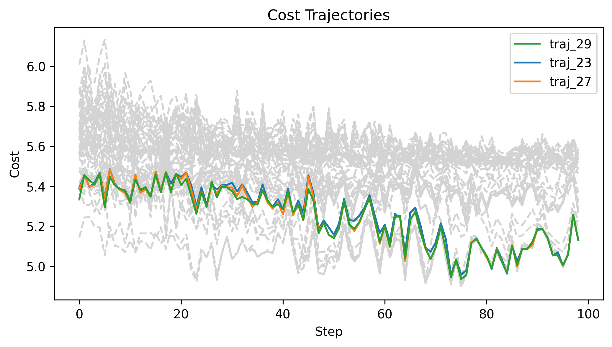
First Order Batch Gradient
Analytic Smoothing of
Contact Dynamics
Gradient Computation
Full state dynamics
Just next object state
Just next object state, but analytically smoothed dynamics
Gradient Computation
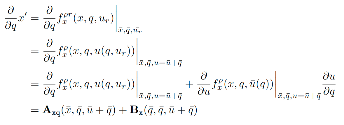
We want to calculate
Analytically smoothed dynamics that takes a relative position command \(u_r\) and only returns \(x\)
Absolute position command as a function of robot position and relative position command
Gradient Computation
Gradient Computation
Gradient Computation
Weighted L2 Norm Cost
Gradient Computation
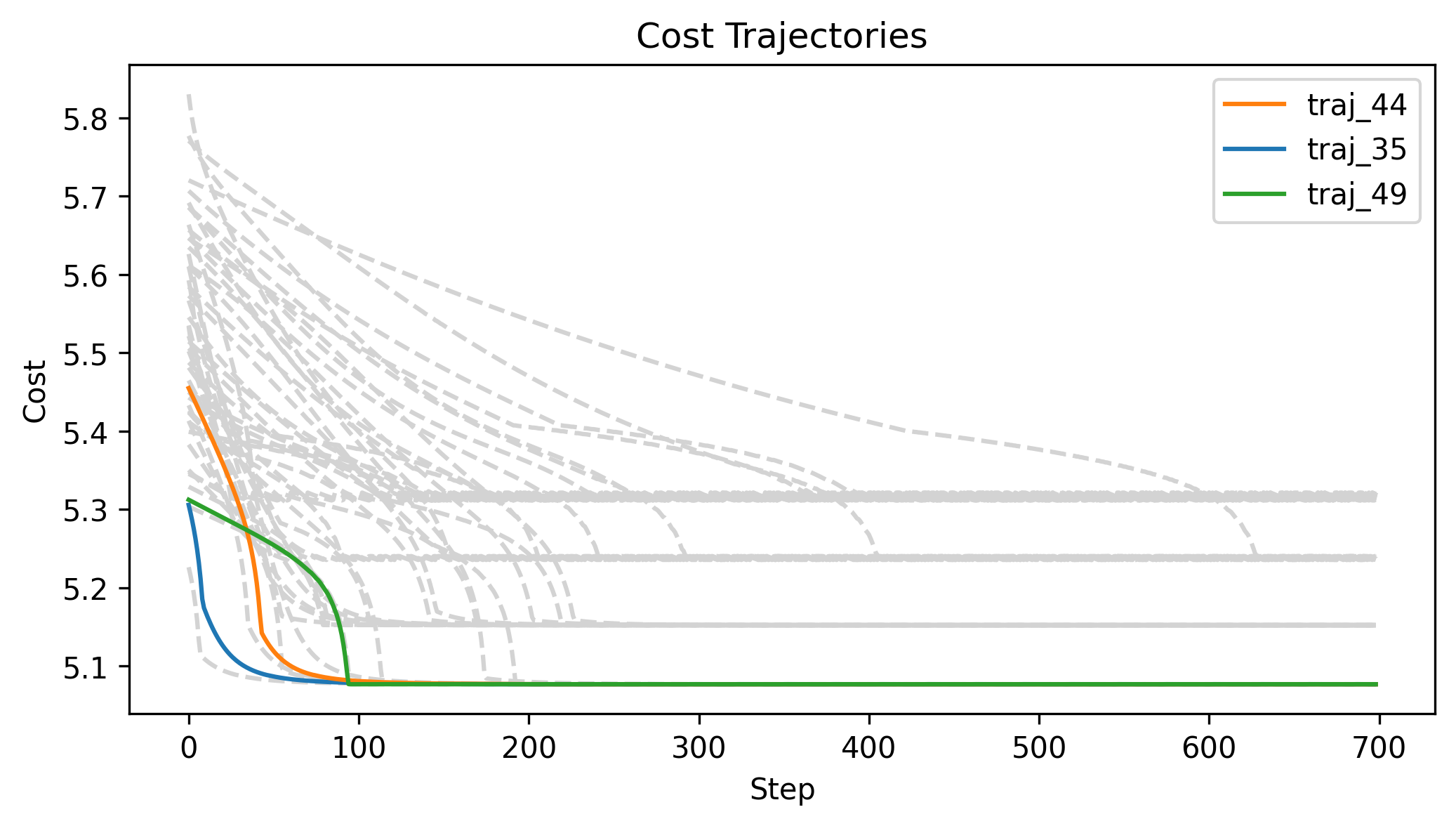
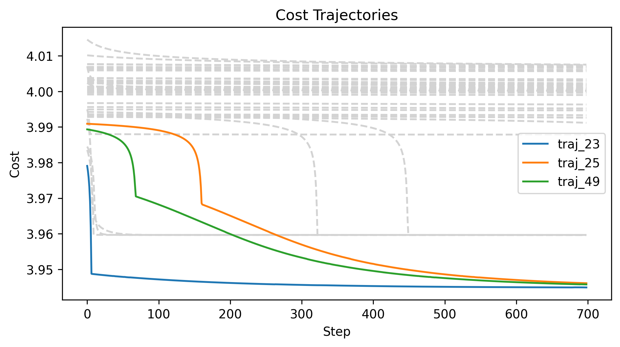
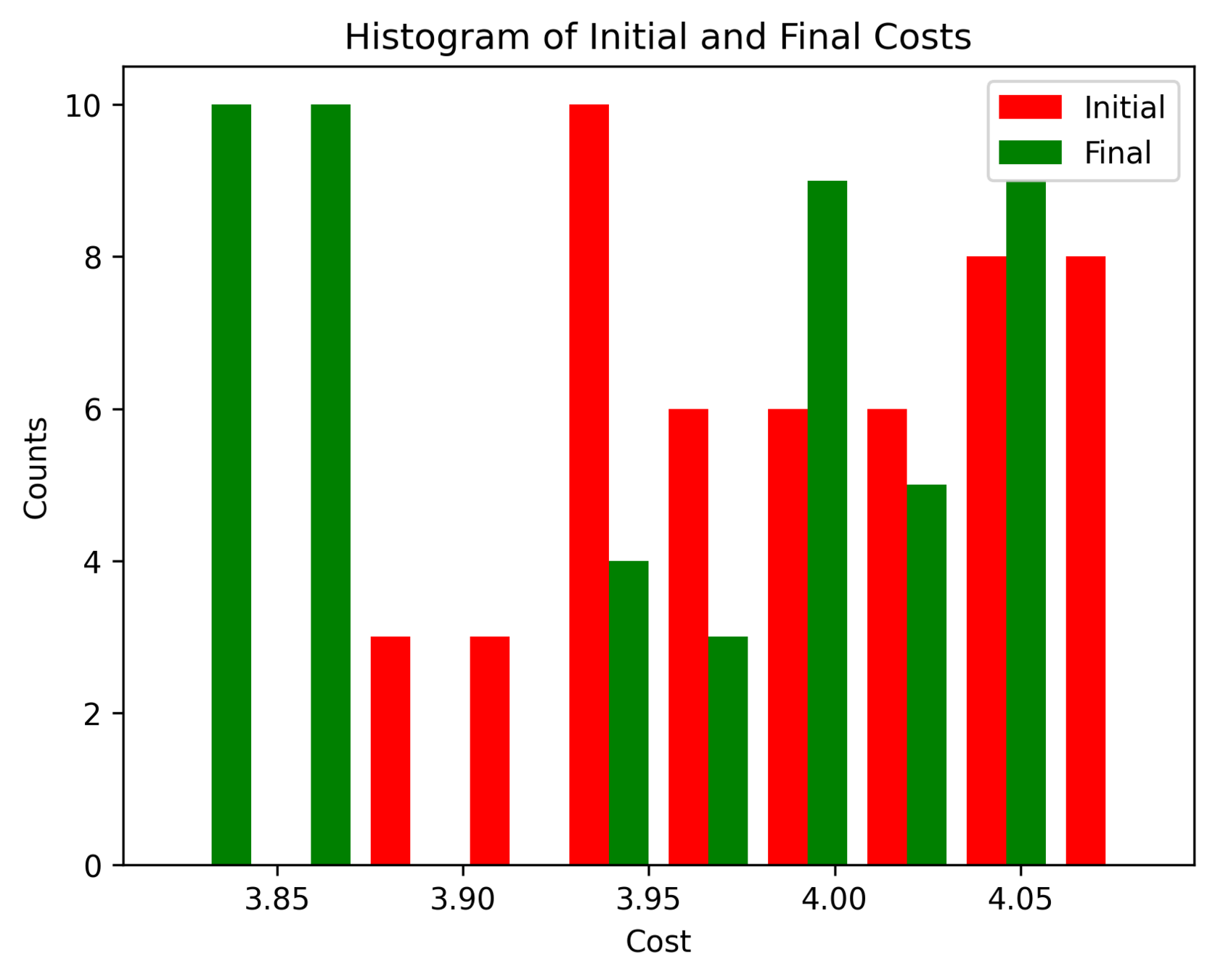
First Order Batch Gradient
\(x_g\) = [-1.5,-1.5,1], log barrier weight = 100, h = 0.01
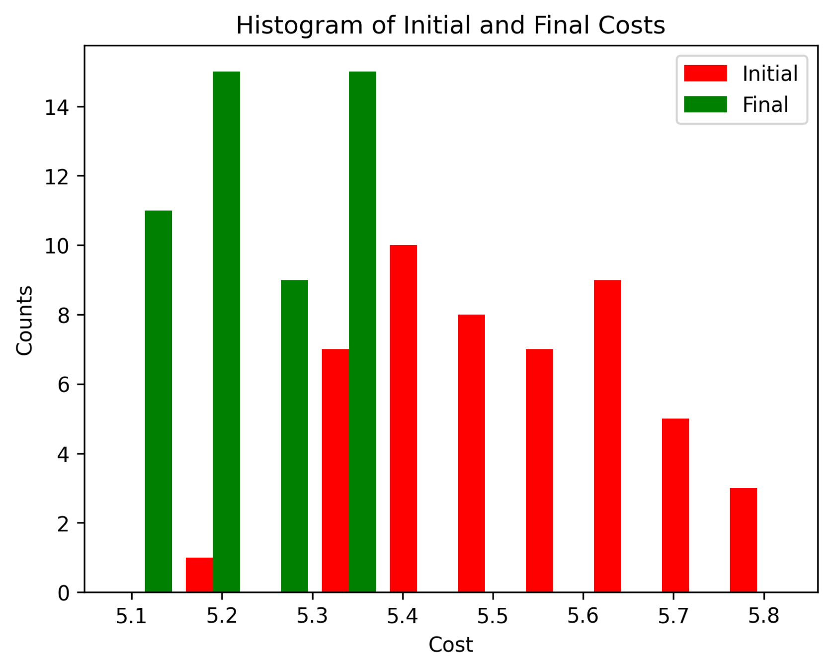
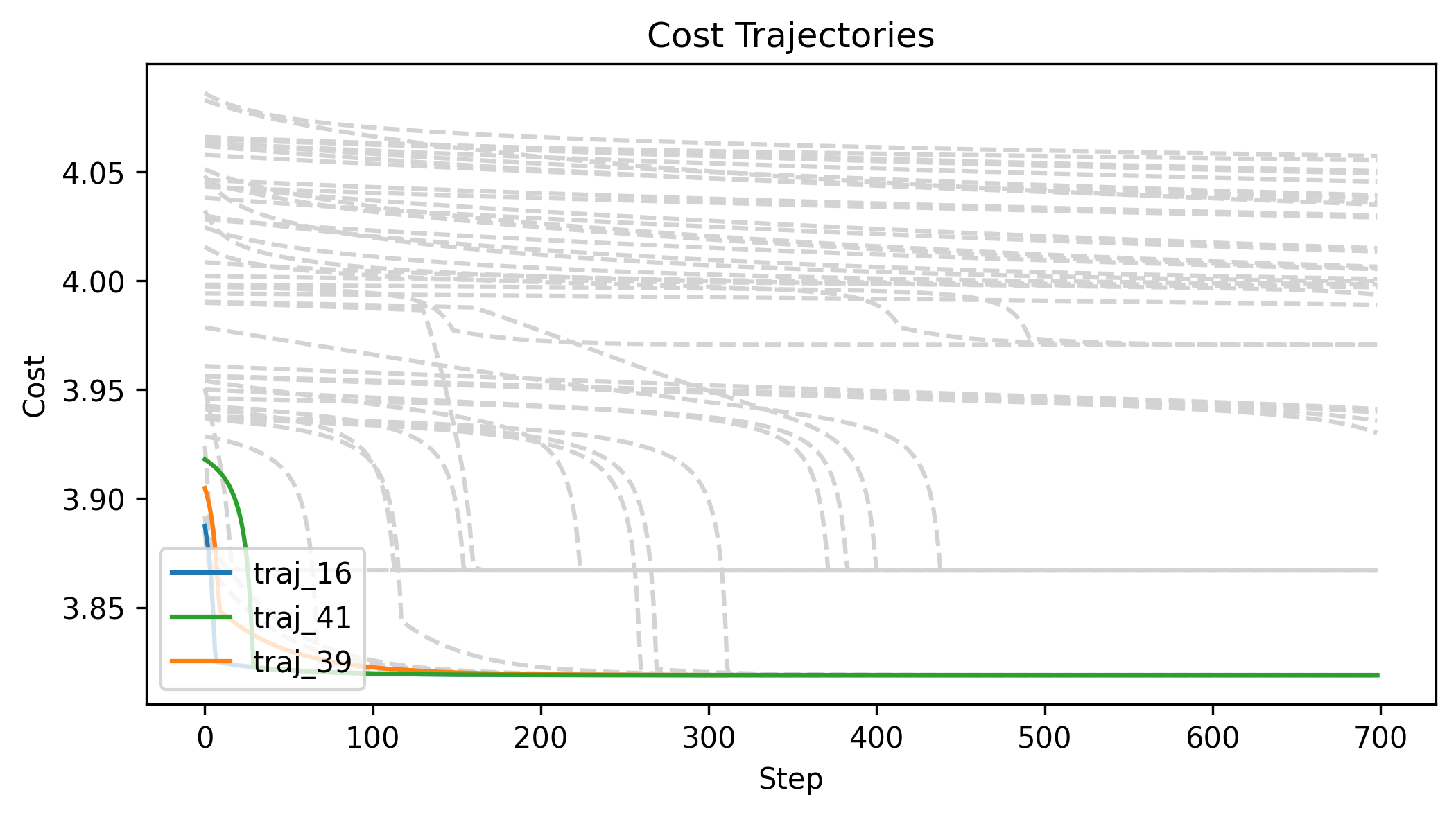
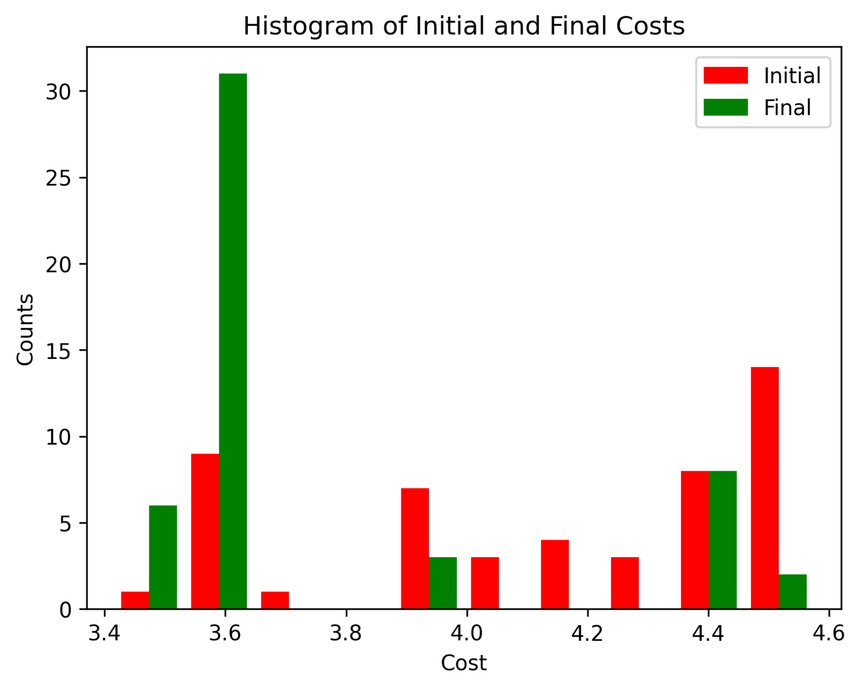
First Order Batch Gradient
\(x_g\) = [-1.5,-1.5,1], log barrier weight = 100, h = 0.01
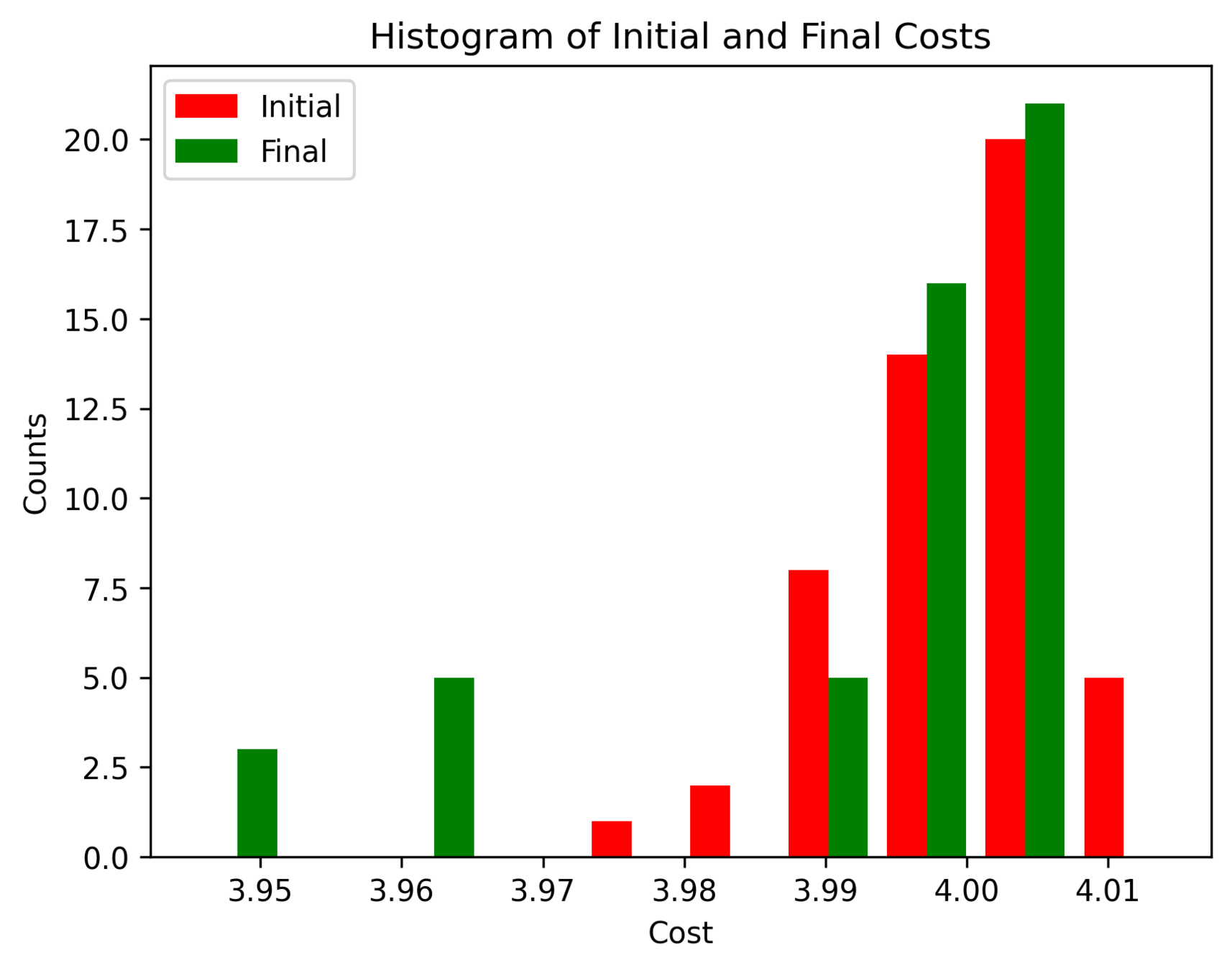
First Order Batch Gradient
\(x_g\) = [-1.5,-1.5,1], log barrier weight = 100, h = 0.01
First Order Batch Gradient
\(x_g\) = [-1.5,-1.5,1]
Log barrier weight = 1000
(0.001N at 1m)
Log barrier weight = 100
(0.01N at 1m)
Log barrier weight = 10
(0.1N at 1m)
First Order Batch Gradient
\(x_g\) = [2, 0, 0]
Log barrier weight = 1000
(0.001N at 1m)
Log barrier weight = 100
(0.01N at 1m)
Log barrier weight = 10
(0.1N at 1m)
First Order Batch Gradient \(x_g\) = [2, 0, 0]
Log barrier weight = 1000
(0.001N at 1m)
Log barrier weight = 100
(0.01N at 1m)
Log barrier weight = 10
(0.1N at 1m)
First Order Batch Gradient
\(x_g\) = [0.3, 0, 0]
Log barrier weight = 1000
(0.001N at 1m)
Log barrier weight = 100
(0.01N at 1m)
Log barrier weight = 10
(0.1N at 1m)
Next Steps
- Understand what's going on in the corners
- Try variance schedule/annealing
- Explore randomized smoothing min?
- Try it on more complex rigid body manipulators (Planar hand, Allegro hand)
- Try it on deformable objects (Plasticine Lab)
- Integrate into RRT