

Lecture 2: Regression and Regularization
Intro to Machine Learning

- Intro to ML
- Regression and Regularization
- Gradient Descent
- Linear Classification
- Features, Neural Networks I
- Neural Networks II (Backprop)
- Convolutional Neural Networks
- Representation Learning
- Transformers
- Markov Decision Processes
- Reinforcement Learning
- Non-parametric Models
6.390 topics in order:
Recall week 1:
- Terminologies:
- Ordinary least squares regression:
- matrix-vector form objective
- closed-form solution
\( J(\theta) =\frac{1}{n}({X} \theta-{Y})^{\top}({X} \theta-{Y})\)
supervised learning
regression
classification
training data
test data
features
label
loss function
training error
test error
hypothesis
hypothesis class
parameters
\(\theta^*=\left({X}^{\top} {X}\right)^{-1} {X}^{\top} {Y}\)
| City | Features | Label | |
|---|---|---|---|
| Temperature | Population | Energy Used | |
| Chicago | 1 | 0 | 2 |
| New York | 0 | 1 | 3 |
| Boston | 1 | 1 | 5 |
training data
Assemble in matrix-vector form:
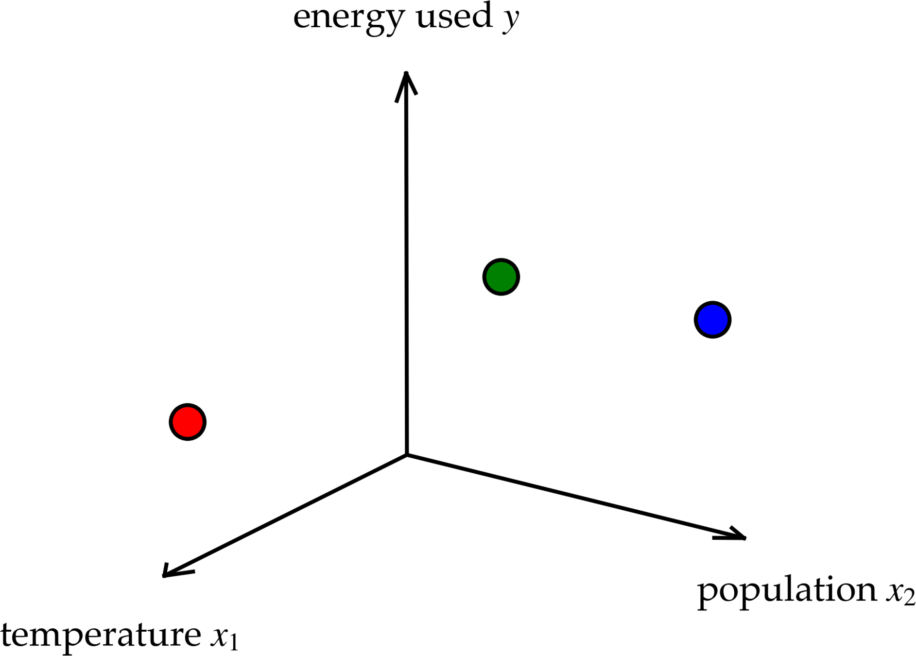
[contrived data]
\(X = \begin{bmatrix} {\color{#cc0000}{1}} & {\color{#cc0000}{0}} \\ {\color{#0000cc}{0}} & {\color{#0000cc}{1}} \\ {\color{#009900}{1}} & {\color{#009900}{1}} \end{bmatrix}\)
\(\in \mathbb{R}^{3 \times 2}\)
features
\(Y = \begin{bmatrix} {\color{#cc0000}{2}} \\ {\color{#0000cc}{3}} \\ {\color{#009900}{5}} \end{bmatrix}\)
\(\in \mathbb{R}^{3 \times 1}\)
label
\(n\)
\(d\)
\(1\)
Regression
Algorithm
💻
\(\in \mathbb{R}^d \)
\(\in \mathbb{R}\)
\(\mathcal{D}_\text{train}\)
What do we want from the algorithm?
A good way to label new features, i.e. a good hypothesis.
hypothesis
learning algorithm
Regression
Algorithm
💻
\(\in \mathbb{R}^d \)
\(\in \mathbb{R}\)
\(\mathcal{D}_\text{train}\)
🧠 ⚙️
The "good"ness depends on human choices, even before the algorithm does anything
hypothesis class
loss function
\(\in \mathbb{R}^d \)
\(\in \mathbb{R}\)
\(\mathcal{D}_\text{train}\)
🧠 ⚙️
linear hypothesis class
squared loss function
Ordinary least squares regression
Regression
Algorithm
💻
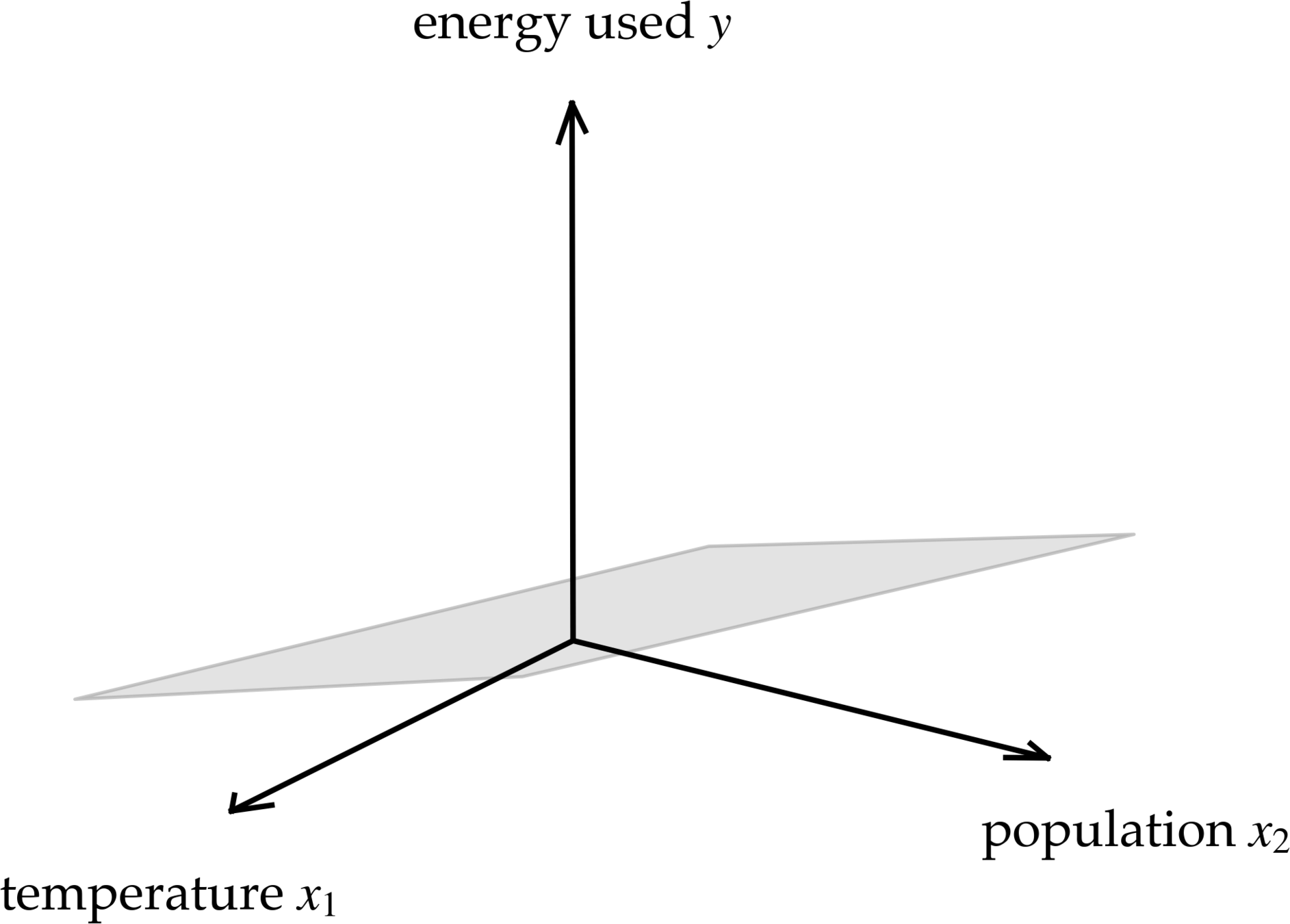
Linear hypothesis class:
\(h(\theta; x) = {\color{#3c78d8}{\begin{bmatrix} \theta_1 & \theta_2 & \cdots & \theta_d \end{bmatrix}}}\begin{bmatrix} x_1 \\ x_2 \\ \vdots \\ x_d \end{bmatrix}\)
parameters
see recitations/labs for how to handle the offset \(\theta_0\)
\(= {\color{#3c78d8}{\theta^\top}}\, x\)
features
Squared loss:
| City | Features | Label | |
|---|---|---|---|
| Temperature | Population | Energy Used | |
| Chicago | 1 | 0 | 2 |
| New York | 0 | 1 | 3 |
| Boston | 1 | 1 | 5 |
\( J(\theta) = \frac{1}{3}\big[ ({\theta_1} \cdot {\color{#cc0000}{1}} + {\theta_2} \cdot {\color{#cc0000}{0}} - {\color{#cc0000}{2}})^2 + ({\theta_1} \cdot {\color{#0000cc}{0}} + {\theta_2} \cdot {\color{#0000cc}{1}} - {\color{#0000cc}{3}})^2 + ({\theta_1} \cdot {\color{#009900}{1}} + {\theta_2} \cdot {\color{#009900}{1}} - {\color{#009900}{5}})^2 \big]\)
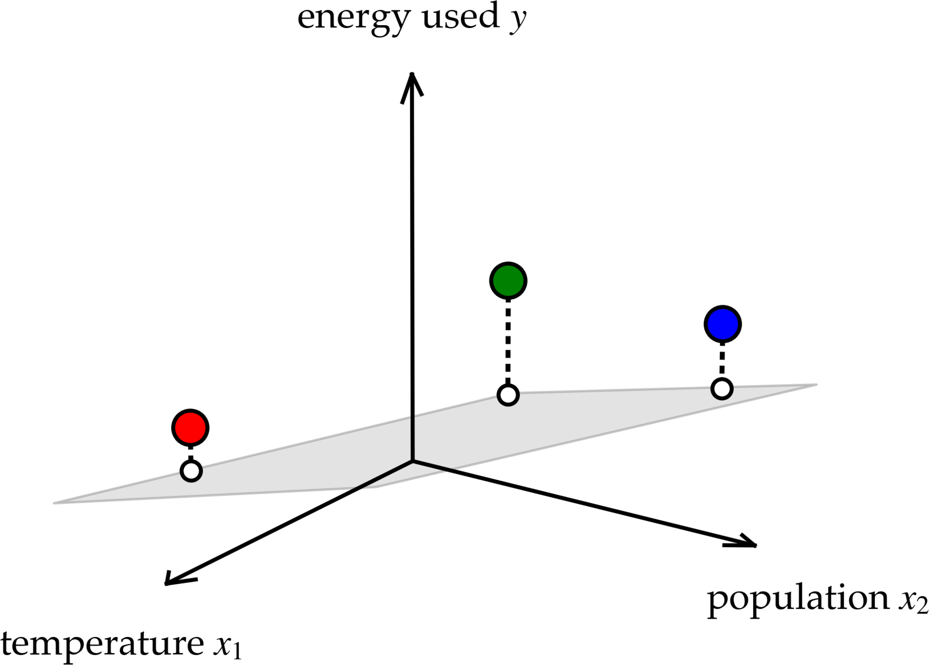
for a given data set, training error only
depends on the parameter
\(X = \begin{bmatrix} {\color{#cc0000}{1}} & {\color{#cc0000}{0}} \\ {\color{#0000cc}{0}} & {\color{#0000cc}{1}} \\ {\color{#009900}{1}} & {\color{#009900}{1}} \end{bmatrix}\)
\(Y = \begin{bmatrix} {\color{#cc0000}{2}} \\ {\color{#0000cc}{3}} \\ {\color{#009900}{5}} \end{bmatrix}\)
\(n=3\)
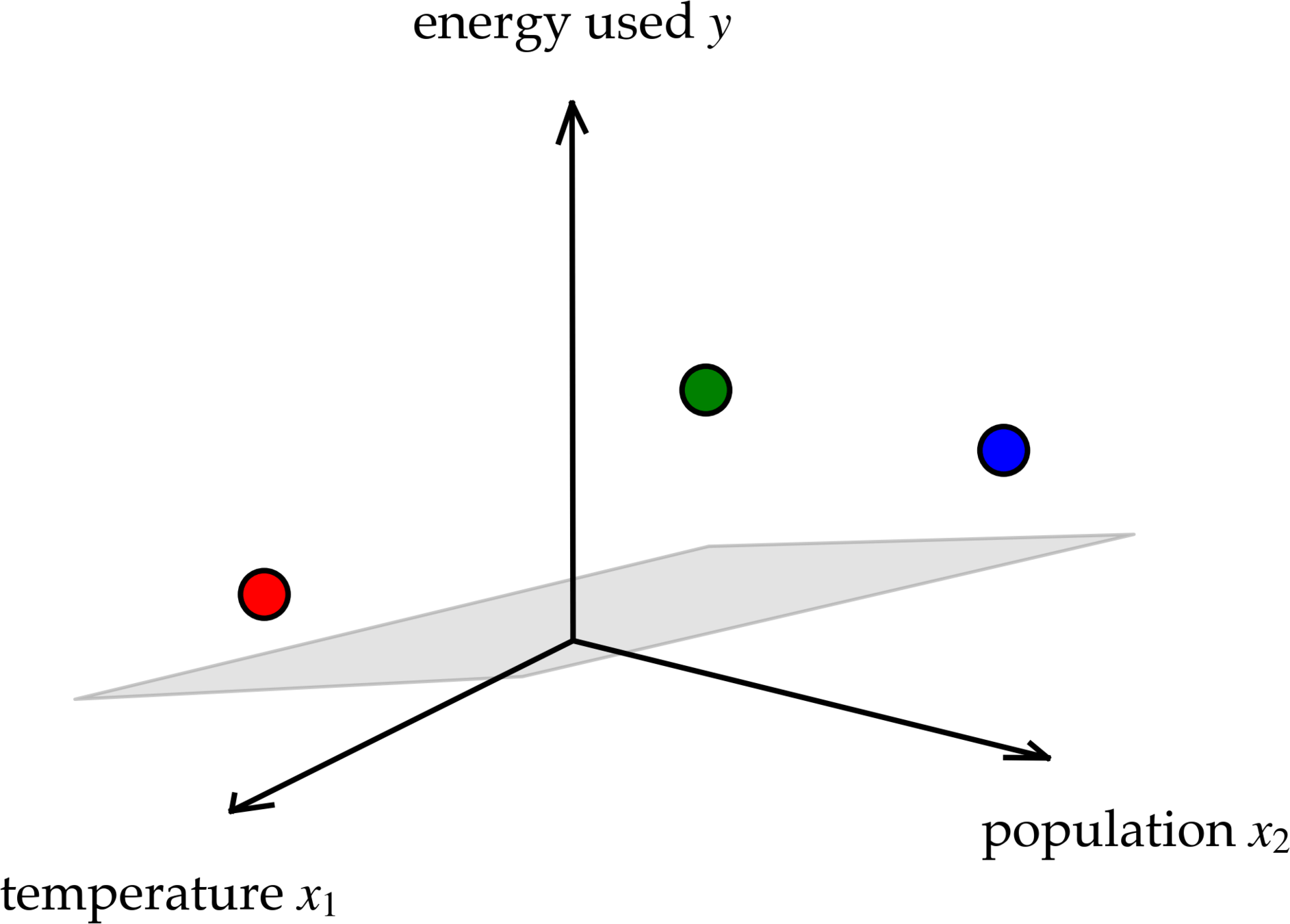
\( J(\theta) =\frac{1}{n}({X} \theta-{Y})^{\top}({X} \theta-{Y})\)
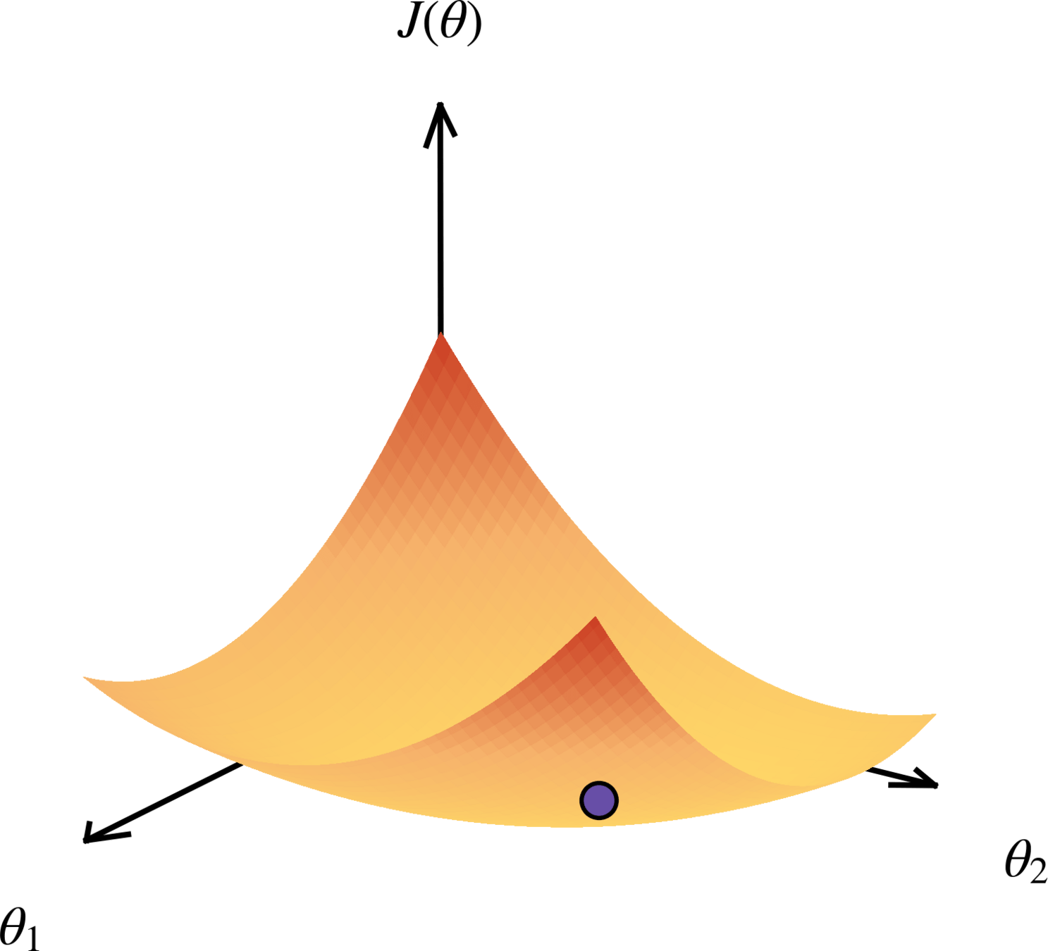
MSE written in matrix-vector form:
\(\theta^*=\left({X}^{\top} {X}\right)^{-1} {X}^{\top} {Y}\)
\(X = \begin{bmatrix} {\color{#cc0000}{1}} & {\color{#cc0000}{0}} \\ {\color{#0000cc}{0}} & {\color{#0000cc}{1}} \\ {\color{#009900}{1}} & {\color{#009900}{1}} \end{bmatrix}\)
\(Y = \begin{bmatrix} {\color{#cc0000}{2}} \\ {\color{#0000cc}{3}} \\ {\color{#009900}{5}} \end{bmatrix}\)
\(n=3\)
\( J(\theta) = \frac{1}{3}\big[ ({\theta_1} \cdot {\color{#cc0000}{1}} + {\theta_2} \cdot {\color{#cc0000}{0}} - {\color{#cc0000}{2}})^2 + ({\theta_1} \cdot {\color{#0000cc}{0}} + {\theta_2} \cdot {\color{#0000cc}{1}} - {\color{#0000cc}{3}})^2 + ({\theta_1} \cdot {\color{#009900}{1}} + {\theta_2} \cdot {\color{#009900}{1}} - {\color{#009900}{5}})^2 \big]\)
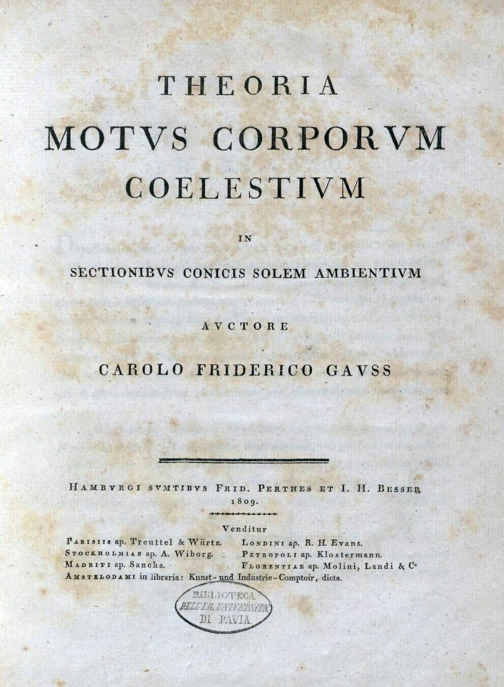
Primary source: Gauss, Theoria motus (1809).
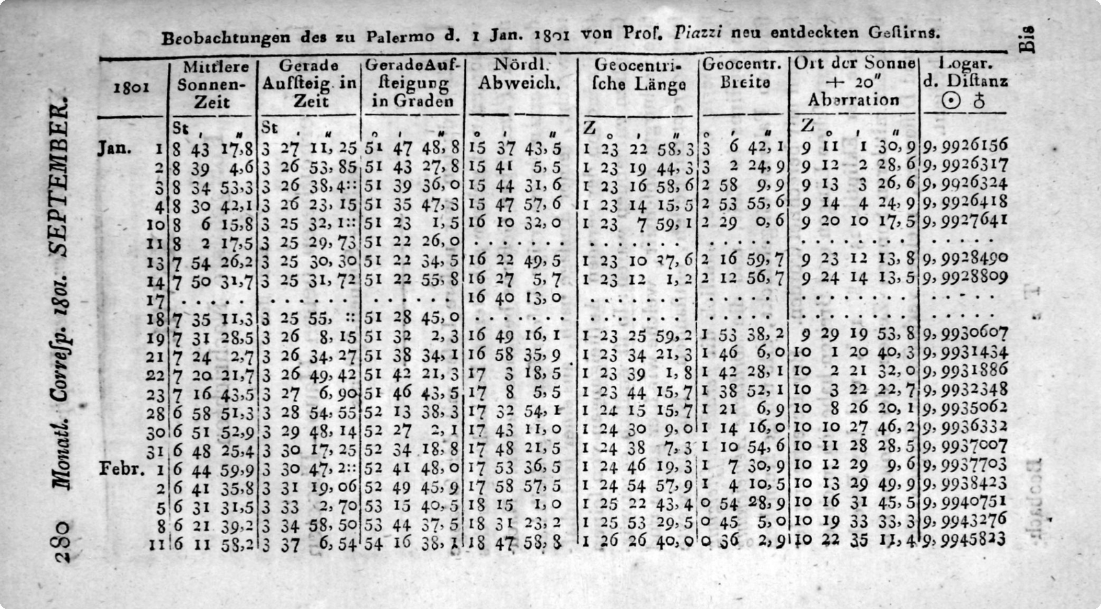
Observation table: Piazzi’s measurements of Ceres (1801).
The beauty of
\(\theta^*=\left({X}^{\top} {X}\right)^{-1} {X}^{\top} {Y}\)
Still a strong baseline in this era of deep learning and agentic AI
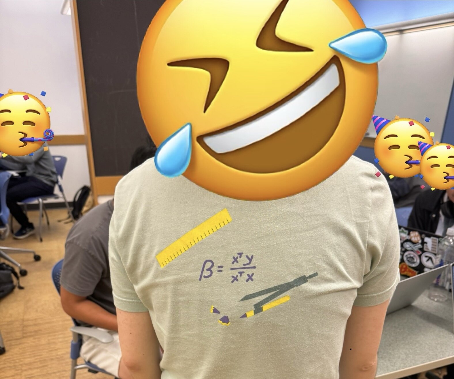
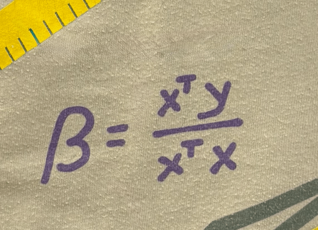
Jane street shirt
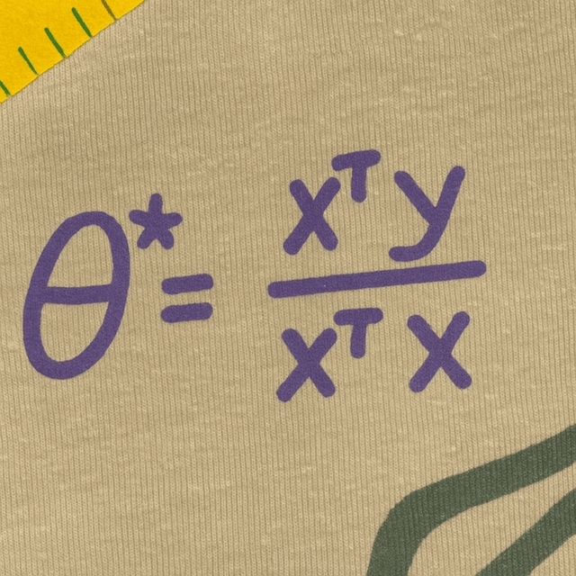
The beauty of
\(\theta^*=\left({X}^{\top} {X}\right)^{-1} {X}^{\top} {Y}\)
why does the shirt formula look different?
shirt formula assumes one-dimensional feature
The beauty of
\(\theta^*=\left({X}^{\top} {X}\right)^{-1} {X}^{\top} {Y}\)
- We solve it in closed form, so it never feels like training.
- This is a rare case where we get a clean, general solution with a theoretical guarantee.
- When well-defined, \(\theta^*\) is the unique minimizer of \(J(\theta)\).
Outline
- The "trouble" with the closed-form solution
- visually, practically, mathematically
- Regularization and ridge regression
- \(\lambda\), a hyperparameter
- Validation and cross-validation
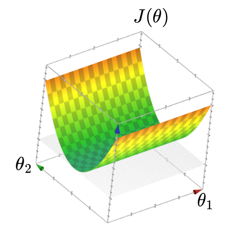
\(\infty\) many optimal \(\theta^*\)
temperature \(x_1\)
population \(x_2\)
energy used
\(y\)
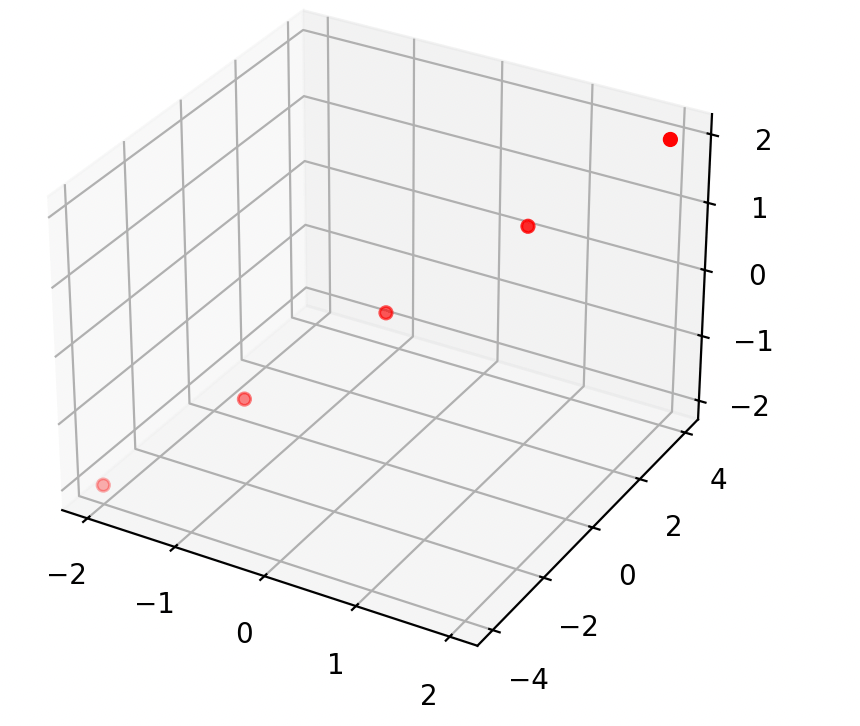
temperature ( °F) \(x_1\)
temperature (°C) \(x_2\)
energy used
\(y\)
data
MSE
\(\theta^*=\left({X}^{\top} {X}\right)^{-1} {X}^{\top} {Y}\)
not well-undefined
(a) \(n < d\)
(b) linearly-dependent features (collinear):
closed-form formula
optimal solution
Not enough info to pin down a unique solution
e.g. genomics, NLP
e.g. temp °F/°C, age/birth_year, ...
\(\left({X}^{\top} {X}\right)\) is singular
\({X}\) is not full column rank
demo (a)
\(n < d\): 1 sample, 2 features
\(X\)
\(X^\top\)
\(=\)
\(\begin{bmatrix}2\\3\end{bmatrix}\)
\(\begin{bmatrix}2 & 3\end{bmatrix}\)
\(= \begin{bmatrix}4 & 6\\6 & 9\end{bmatrix}\)
demo (b)
collinear: \(x_2 = 1.5 \cdot x_1\)
\(X\)
\(X^\top\)
\(=\)
\(\begin{bmatrix}2 & 4 & 6\\3 & 6 & 9\end{bmatrix}\)
\(\begin{bmatrix}2 & 3\\4 & 6\\6 & 9\end{bmatrix}\)
\(= \begin{bmatrix}56 & 84\\84 & 126\end{bmatrix}\)
mathematically, formula not well-defined when:
- That formula is not well-defined 👉
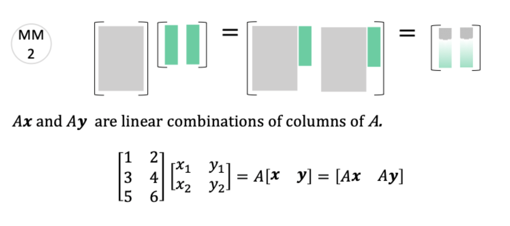
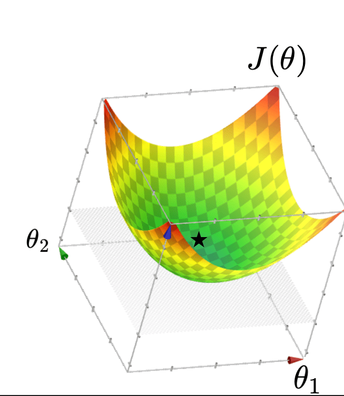
Typically, \(X\) is full column rank
- \(\theta^*=\left({X}^{\top} {X}\right)^{-1} {X}^{\top} {Y}\)
- \(J(\theta)\) "curves up" everywhere
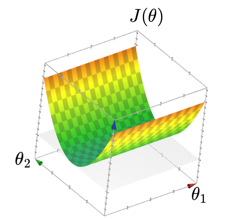
When \(X\) is not full column rank
- \(J(\theta)\) has a "flat" bottom
- Infinitely many optimal hyperplanes
- unique optimal hyperplane
\(X^\top X\) "invertibility"
(the formula isn't wrong; data is trouble-making 🥺)
\(X^\top X\) singular
e.g., single 1d data point \((x,y\))
formula simplifies to \(\theta^*=\frac{y}{x}\)
When \(X^\top X\) is almost singular:
\(\theta^*=\left({X}^{\top} {X}\right)^{-1} {X}^{\top} {Y}\) technically is well-defined
\(\theta^*\) tends to have huge magnitude and very sensitive to the data
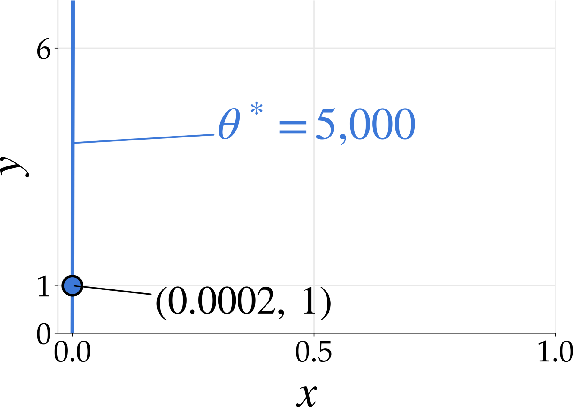
\(X = \begin{bmatrix}-2 & -4.00006\\-1 & -2.00004\\1 & 2.00004\\2 & 4.00006\end{bmatrix}\)
\(Y = \begin{bmatrix}-1.8\\-1.2\\1.2\\1.8\end{bmatrix}\)
formula gives \(\theta^* \approx \begin{bmatrix}-60000\\30000\end{bmatrix}\)
e.g.,
if the 2nd feature changes by 0.1, prediction changes 3000
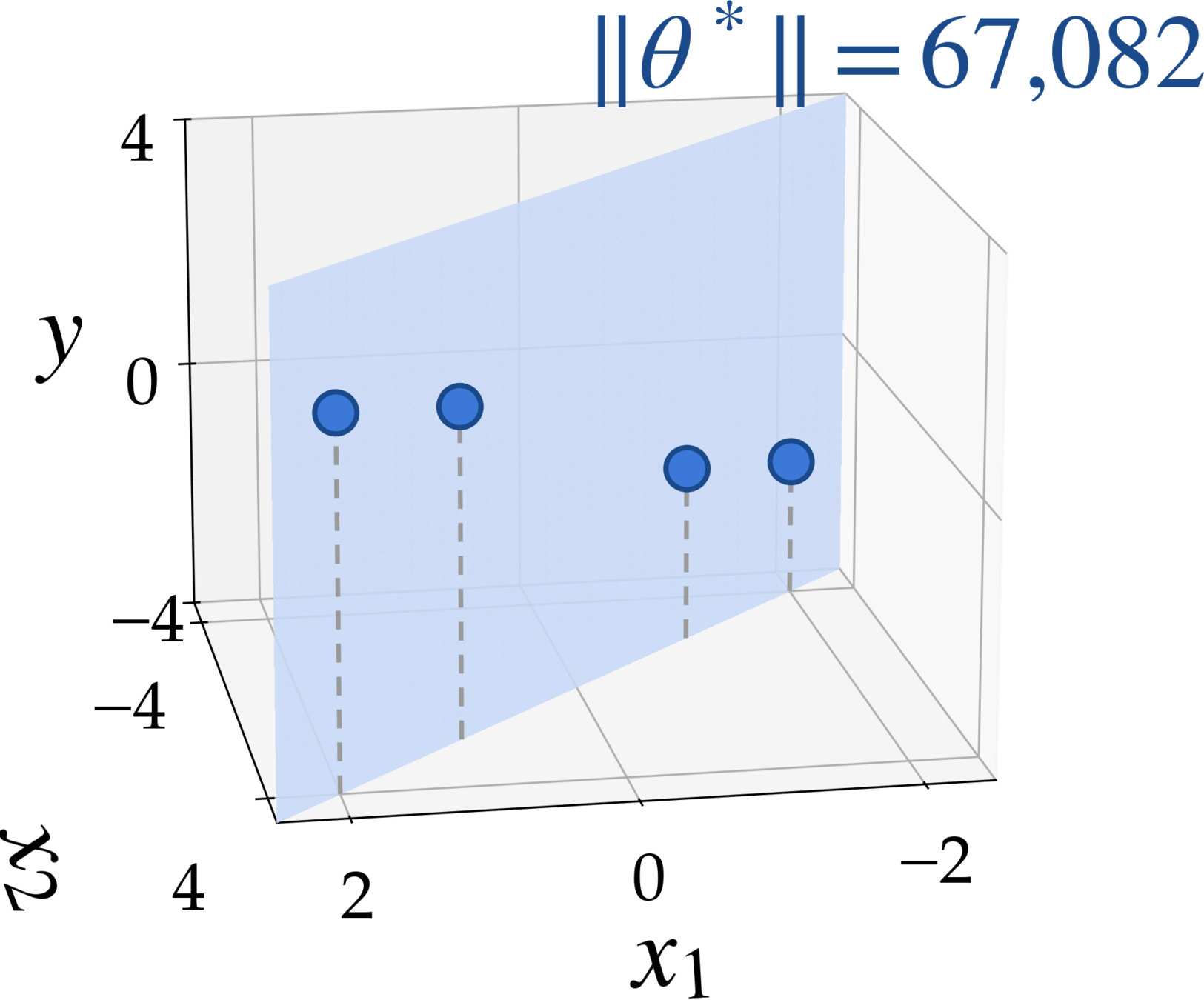
meanwhile, lots of other \(\theta\)s fit the training data very well too
\(\theta^*=\left({X}^{\top} {X}\right)^{-1} {X}^{\top} {Y}\) technically exists and is the unique optimal
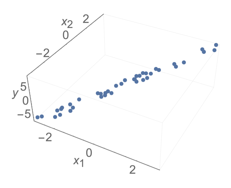
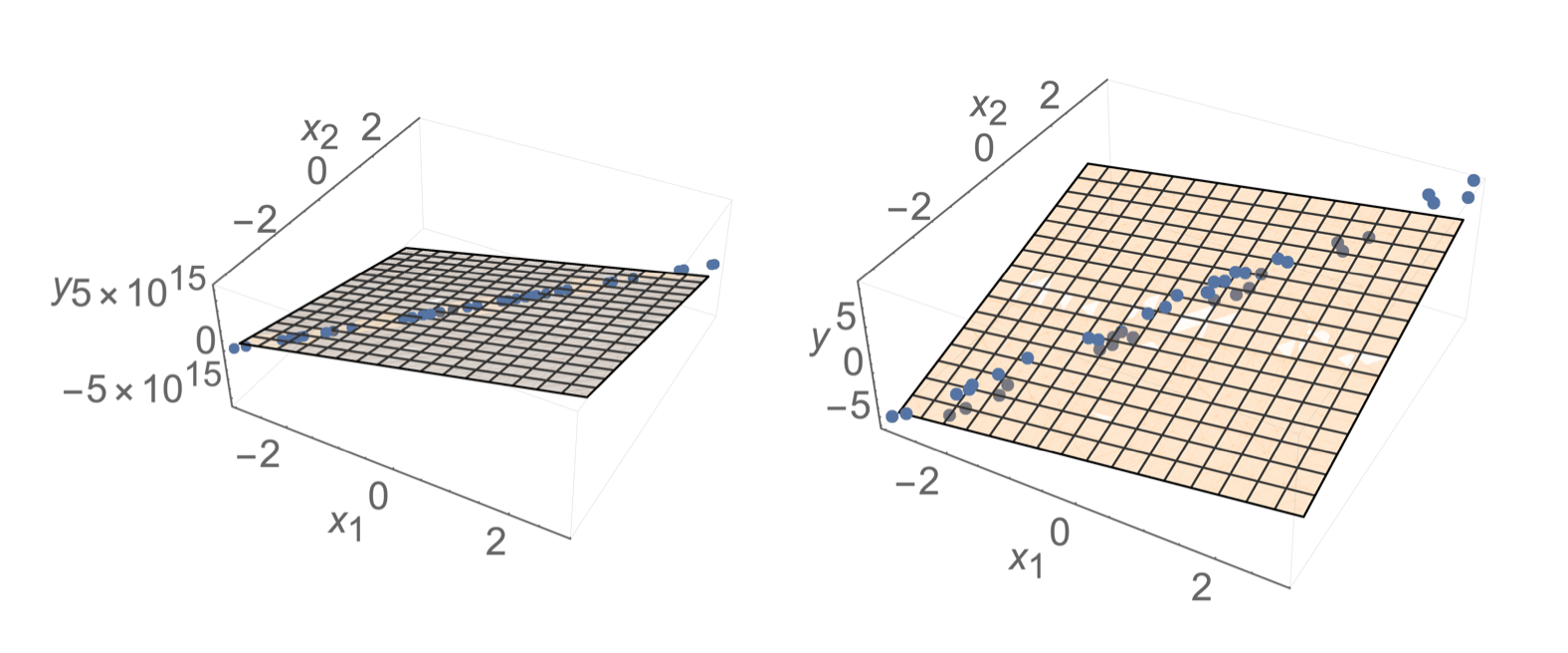
when \(X^\top X\) is almost singular
lots of other \(\theta\)s fit the training data very well too
🥺
\(\theta^*\) tends to have huge magnitude and very sensitive to the data
\(\theta^*\) tends to overly cater to the training data --- overfitting
Outline
- The "trouble" with the closed-form solution
- Regularization and ridge regression
- \(\lambda\), a hyperparameter
- Validation and cross-validation
Ridge regularization
\(\lambda\) controls how heavily we penalize magnitude relative to MSE
for the given training data set (so \(X, Y, n\) are constants) and a given \(\lambda>0\):
still searching for parameters \(\theta\)
How does \(\lambda\) affect the learned \(\theta\)?
- \(\lambda = 0\)?
- \(\lambda = 1000\)?
- \(\lambda = -100\)?
- No penalty — reduces to MSE
- Huge penalty — forces \(\theta \approx 0\)
- Rewards large \(\theta\) — counter-productive! ¹
1. this is why we require \(\lambda > 0\)
Ridge objective
alleviates overfitting by sacrificing MSE
Ridge solution
2. for \(\lambda > 0\): \(\theta^*_{\text{ridge}}\) always exists and is unique
Regression
Algorithm
💻
\(\in \mathbb{R}^d \)
\(\in \mathbb{R}\)
\(\mathcal{D}_\text{train}\)
🧠 ⚙️
- hypothesis class
- loss function
- hyperparameter
\(\lambda\) is a hyperparameter
- affects learning outcome, and not learned by minimizing the training error
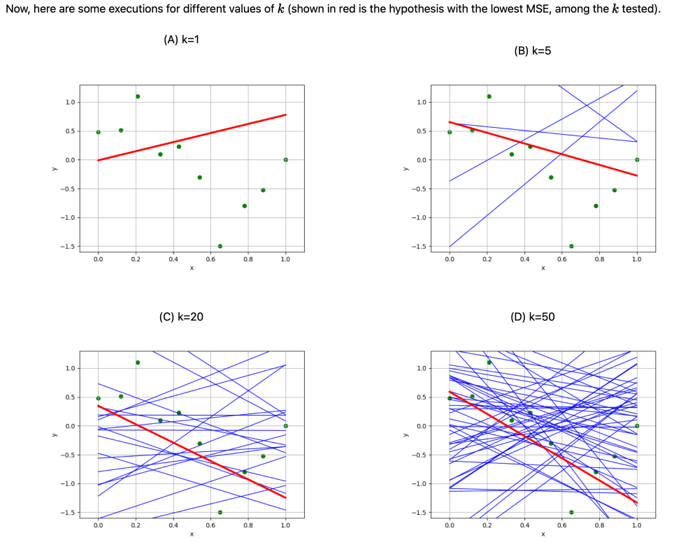
- we already saw a hyperparameter (the number of random regressor in lab1)
Outline
- The "trouble" with the closed-form solution
- Regularization and ridge regression
- \(\lambda\), a hyperparameter
- Validation and cross-validation
We need to choose hyperparameters (like \(\lambda\))
\(\left\{\left(x^{(1)}, y^{(1)}\right), \dots, \left(x^{(n)}, y^{(n)}\right)\right\}\)
\(\mathcal{D}_\text{val}\)
\(\mathcal{D}_\text{train}\)
1. Hold-out some data
- Use \(\mathcal{D}_{\text{val}}\) on \({h_{\lambda}}\) for that \(\lambda\)'s evaluation error
2. For a fixed \(\lambda\):
- Use \(\mathcal{D}_{\text{train}}\) to train a \({h_{\lambda}}\)
3. Repeat step 2 for a bunch of \(\lambda\) candidates, keep track of their evaluation errors
4. pick the \(\lambda\) candidate that led to the lowest evaluation error
Regression
Algorithm
💻
🧠 ⚙️
- linear hypothesis
- ridge objective
- a fixed \(\lambda\)
train on \(\mathcal{D}_{\text{train}}\) with \(\lambda\)
compute \(\mathcal{E}_{\text{val}}(\lambda)\) on \(\mathcal{D}_{\text{val}}\)
for each \(\lambda \):
train on \(\mathcal{D}_{\text{train}}\) with \(\lambda\)
compute \(\mathcal{E}_{\text{val}}(\lambda)\) on \(\mathcal{D}_{\text{val}}\)
return \(\lambda^* = \arg\min_\lambda \mathcal{E}_{\text{val}}(\lambda)\)
\(\mathcal{D}_\text{val}\)
\(\mathcal{D}_\text{train}\)
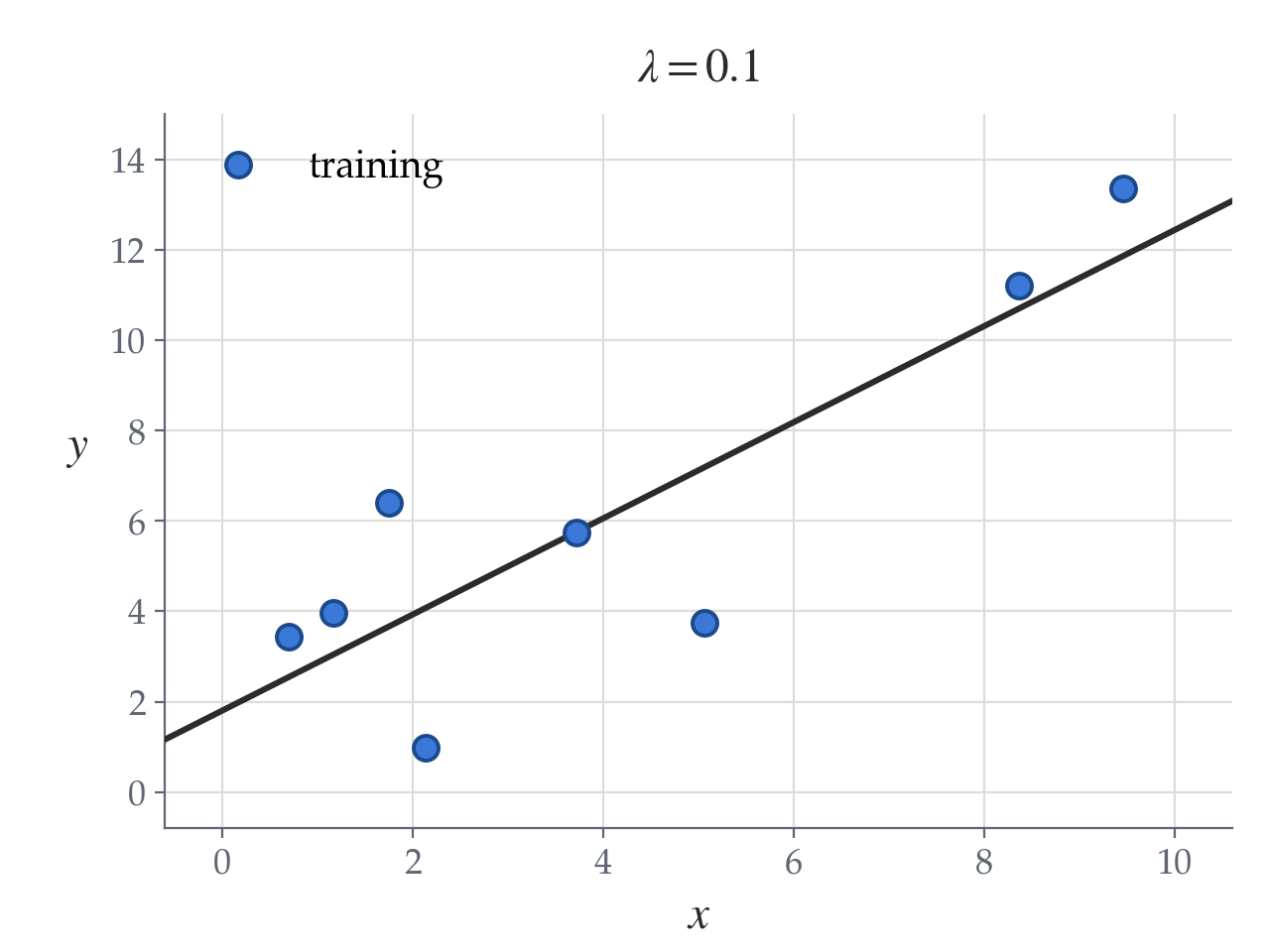
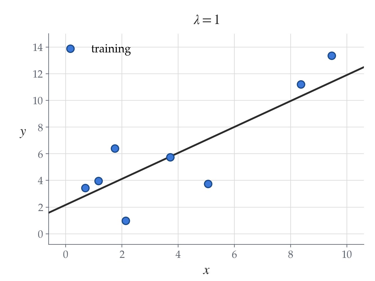
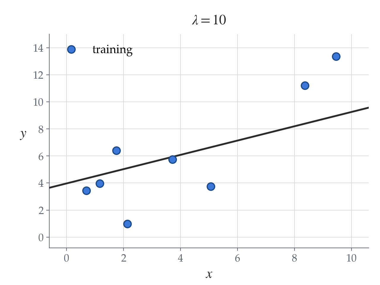
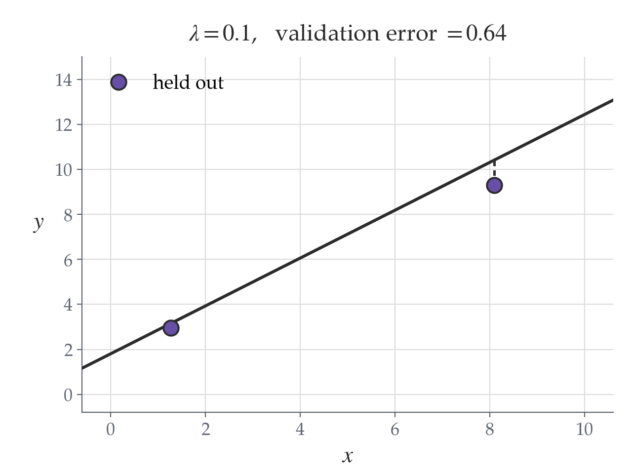
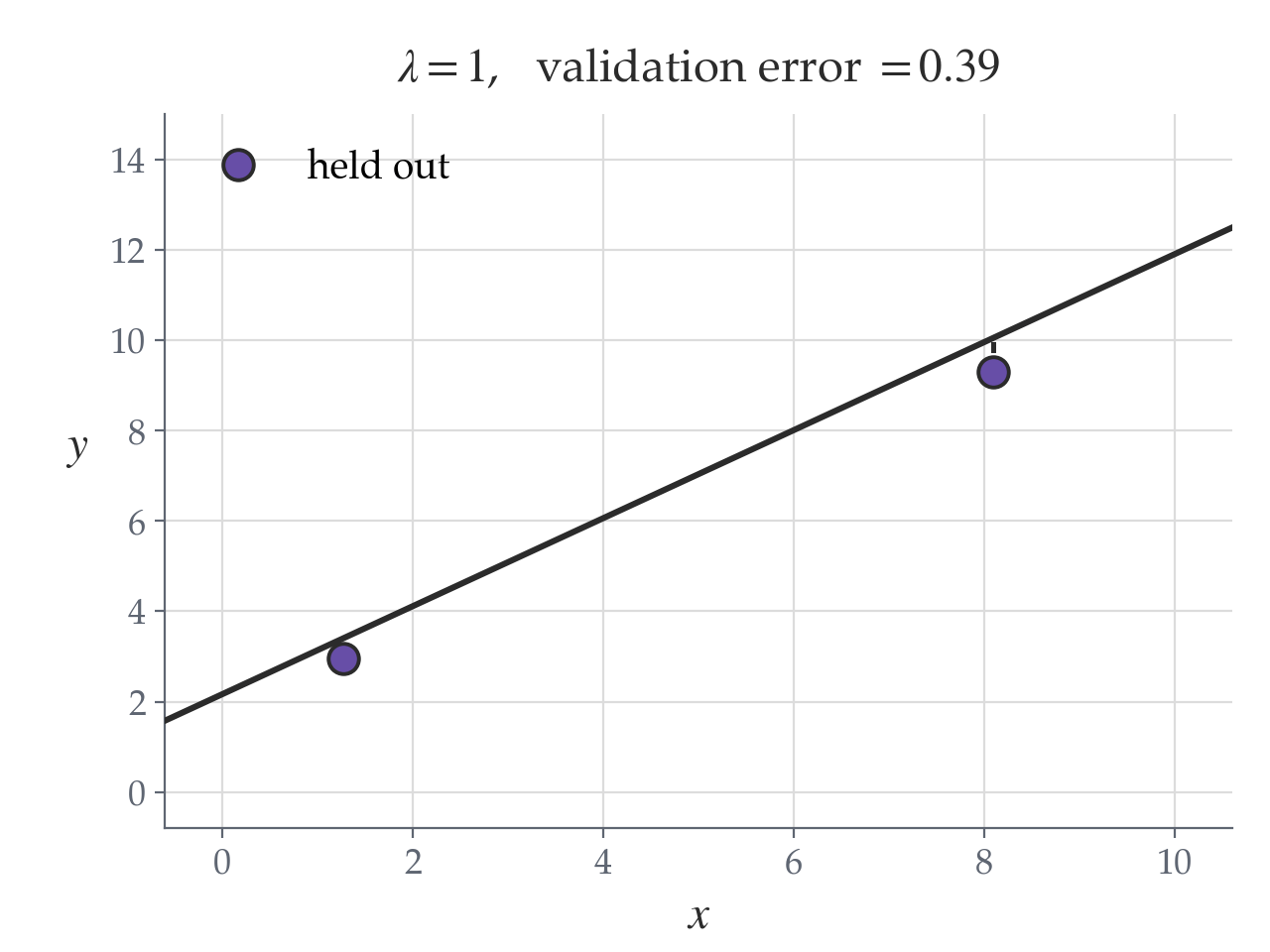
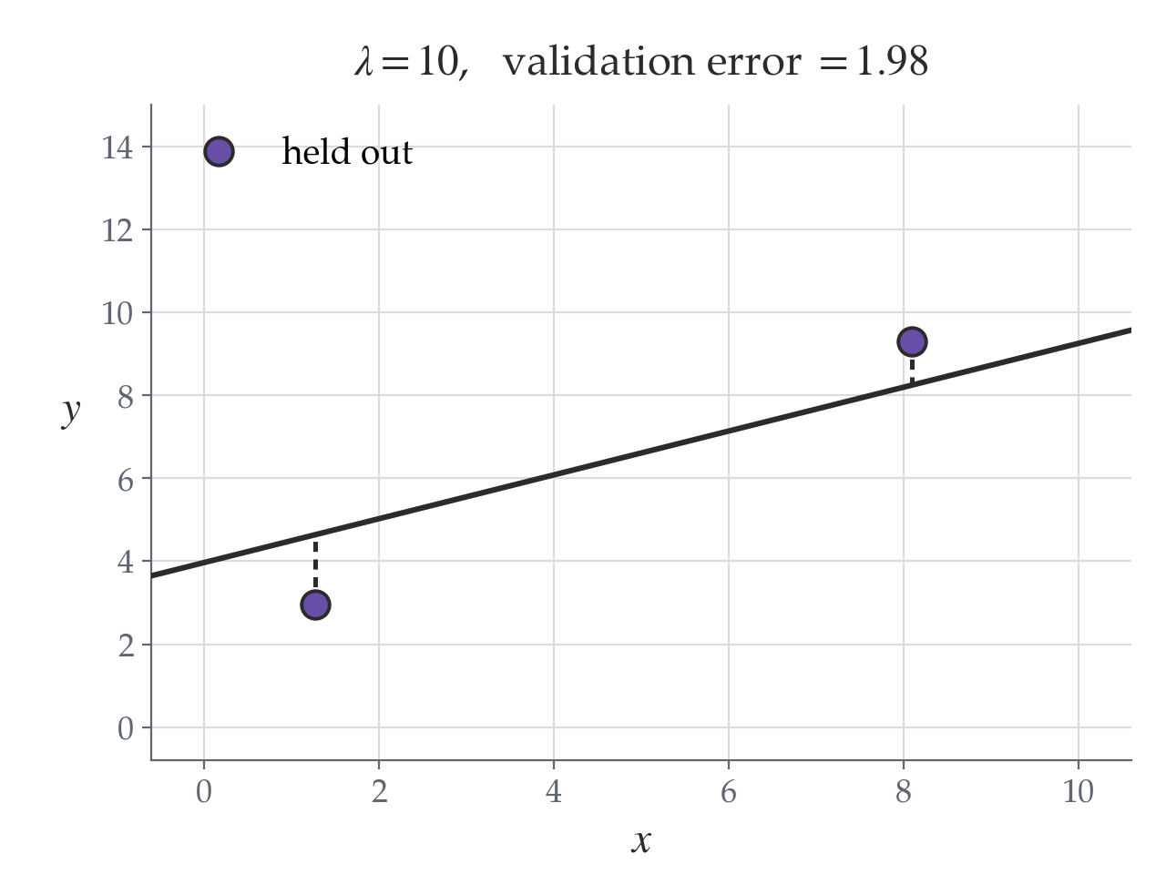
\(\lambda=1\) "wins" as \(\lambda^*\),
\(\theta^*_{\text{final}} = (X^\top X + n \lambda^* I)^{-1} X^\top Y\)
using all 10 data points
train:
validate:
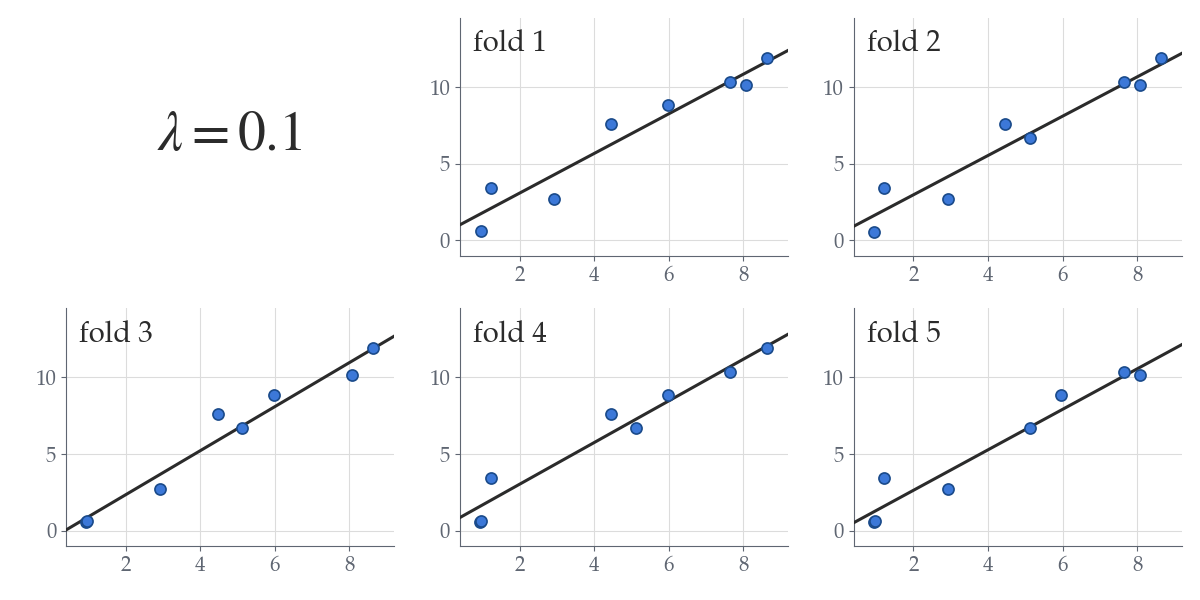
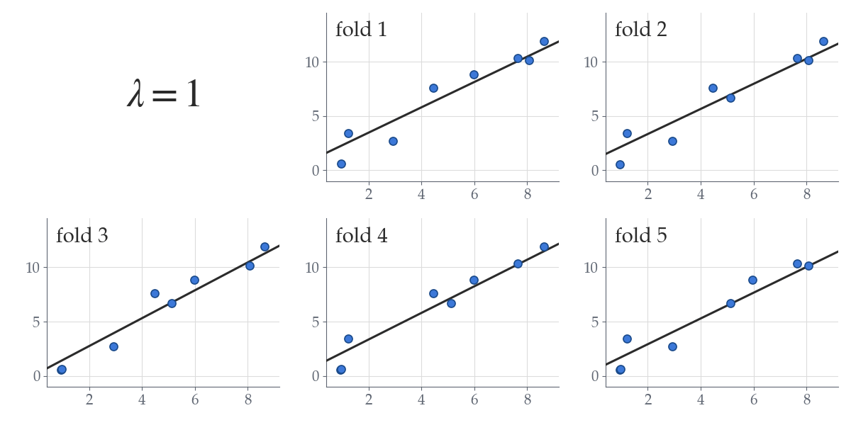
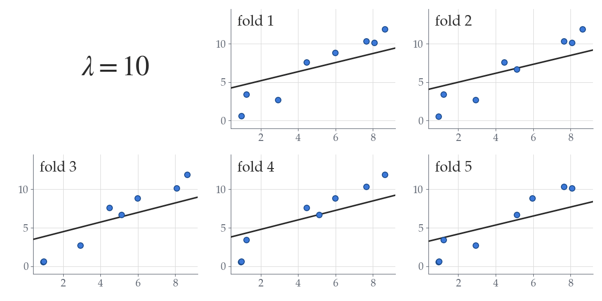
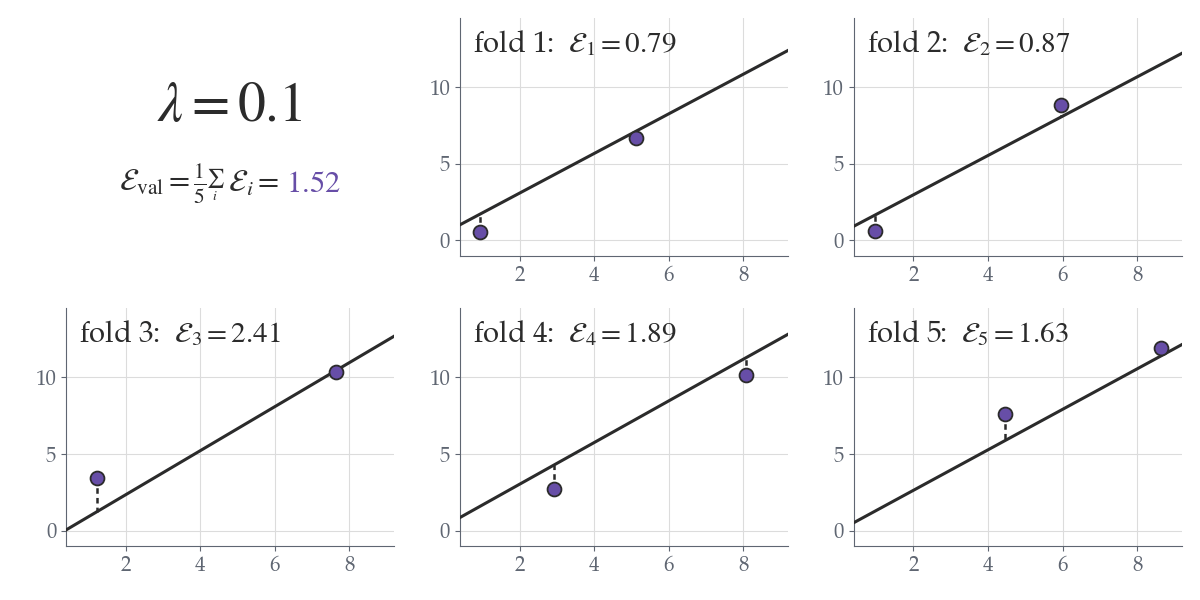
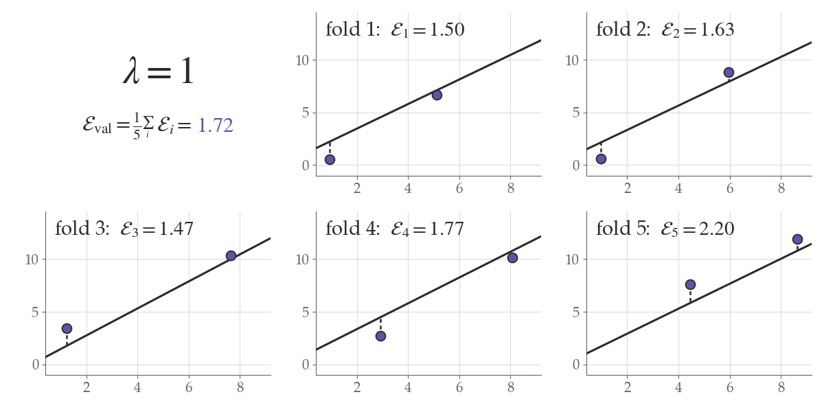
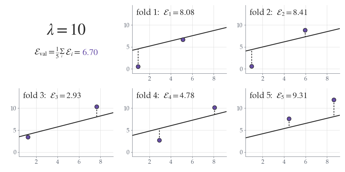
\(K\)-fold cross-validation
for \(i = 1, \dots, 5\):
train \(h_i\) on \(\mathcal{D} \setminus \mathcal{D}_i\) with \(\lambda\)
\(\mathcal{E}_i =\) error on \(\mathcal{D}_i\)
for \(i = 1, \dots, 5\):
train \(h_i\) on \(\mathcal{D} \setminus \mathcal{D}_i\) with \(\lambda\)
\(\mathcal{E}_i =\) error on \(\mathcal{D}_i\)
\(\mathcal{E}_{\text{val}}(\lambda) = (\mathcal{E}_1 + \cdots + \mathcal{E}_5) / 5\)
for each \(\lambda \in \{0.1, 1, 10\}\):
for \(i = 1, \dots, 5\):
train \(h_i\) on \(\mathcal{D} \setminus \mathcal{D}_i\) with \(\lambda\)
\(\mathcal{E}_i =\) error on \(\mathcal{D}_i\)
\(\mathcal{E}_{\text{val}}(\lambda) = (\mathcal{E}_1 + \cdots + \mathcal{E}_5) / 5\)
return \(\lambda^* = \arg\min_\lambda\,\mathcal{E}_{\text{val}}(\lambda)\)
for each \(\lambda \in \{0.1, 1, 10\}\):
for \(i = 1, \dots, 5\):
train \(h_i\) on \(\mathcal{D} \setminus \mathcal{D}_i\) with \(\lambda\)
\(\mathcal{E}_i =\) error on \(\mathcal{D}_i\)
\(\mathcal{E}_{\text{val}}(\lambda) = (\mathcal{E}_1 + \cdots + \mathcal{E}_5) / 5\)
return \(\lambda^* = \arg\min_\lambda\,\mathcal{E}_{\text{val}}(\lambda)\)
outer loop of \(\lambda \in \{0.1, 1, 10\}\):
\(\mathcal{E}_{\text{val}}(\lambda) = (\mathcal{E}_1 + \mathcal{E}_2 + \mathcal{E}_3 + \mathcal{E}_4 + \mathcal{E}_5) / 5\)
How many hypotheses trained in this example to pick \(\lambda^*\)?





e.g., 5-fold, and 3 \(\lambda\) candidates:
\(\lambda=0.1\) "wins" as \(\lambda^*\),
\(\theta^*_{\text{final}} = (X^\top X + n \lambda^* I)^{-1} X^\top Y\)
using all 10 data points
train:
validate:
Summary
singular
full column rank
regularization
ridge regression
hyperparameter
overfitting
validation data
cross-validation
K-fold
-
When \(X^\top X\) is singular, OLS has multiple minimizers.
-
When \(X^\top X\) is nearly singular (ill-conditioned), fitted parameters and predictions are sensitive to small changes in data.
-
Regularization combats overfitting by penalizing large \(\theta\).
-
Ridge regression adds \(\lambda\|\theta\|^2\) to the objective — still has a closed-form solution.
-
\(\lambda\) is a hyperparameter that trades off fit vs. regularization.
-
Validation and cross-validation provide principled ways to choose \(\lambda\).