

Lecture 4: Linear Classification
Intro to Machine Learning

Recall:
"Use" a model
"Learn" a model
Regression
Algorithm
\(\mathcal{D}_\text{train}\)
🧠⚙️
hypothesis class
loss function
hyperparameters
regressor
"Use" a model
"Learn" a model
train, optimize, tune, adapt ...
adjust/update/find \(\theta\)
gradient-based
Regression
Algorithm
\(\mathcal{D}_\text{train}\)
🧠⚙️
hypothesis class
loss function
hyperparameters
regressor
predict, test, evaluate, infer ...
plug in the \(\theta\) found
no gradients involved
Recall:
Today:
{"good", "better", "best", ...}
\(\{0,1\}\)
\(\{😍, 🥺\}\)
{"fish", "grizzly", "chameleon", ...}
Classification
Algorithm
🧠⚙️
hypothesis class
loss function
hyperparameters
classifier
\(\mathcal{D}_\text{train}\)
Outline
- Linear (binary) classifiers
- to use: separator, normal vector
- to learn: no gradient to follow
- Linear logistic (binary) classifiers
- Linear multi-class classifiers
-
Linear (binary) classifiers
- to use: separator, normal vector
- to learn: no gradient to follow
- Linear logistic (binary) classifiers
- Linear multi-class classifiers
linear regressor
linear binary classifier
features
parameters
linear combo
predict
\(x \in \mathbb{R}^d\)
\(\theta \in \mathbb{R}^d, \theta_0 \in \mathbb{R}\)
\(\theta^T x +\theta_0\)
\(g = z\)
\(=z\)
if \(z > 0\)
otherwise
\(1\)
\(0\)
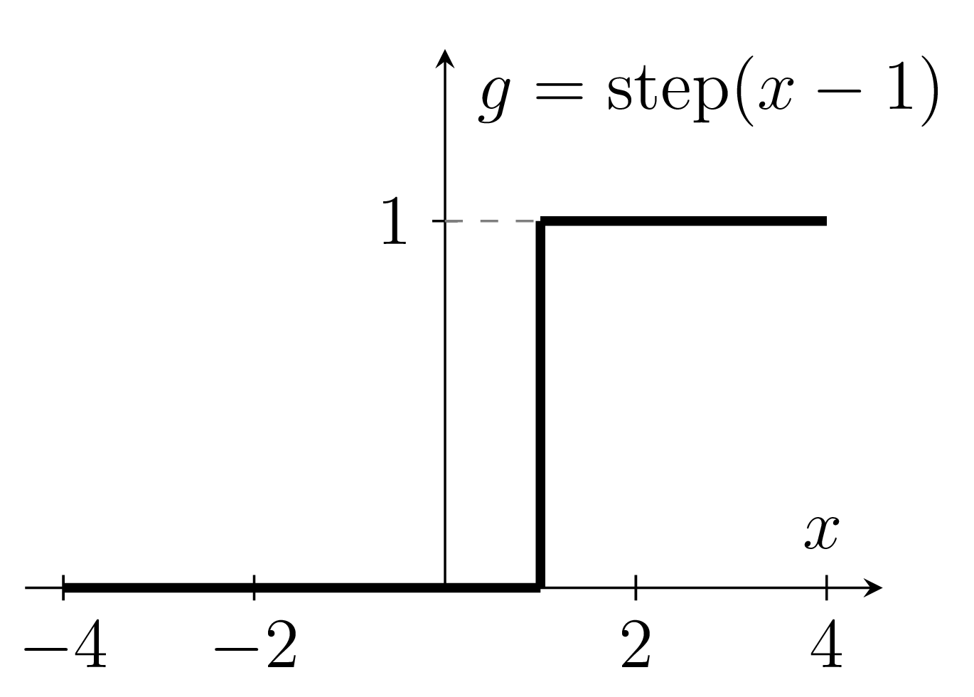
Today, \(z\) stands for \(\theta^T x +\theta_0\).
\(g=\)
label
\(y\in \mathbb{R}\)
\(y\in \{0,1\}\)
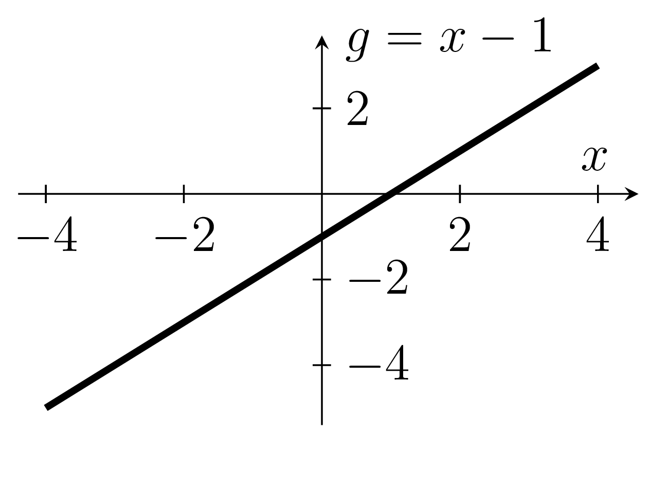
e.g., \(\theta = 1,\ \theta_0 = -1\)
Outline
-
Linear (binary) classifiers
- to use: separator, normal vector
- to learn: no gradient to follow
- Linear logistic (binary) classifiers
- Linear multi-class classifiers
- To learn a model, we need a loss function.
- Very intuitive and easy to evaluate 😍
- One natural loss choice:
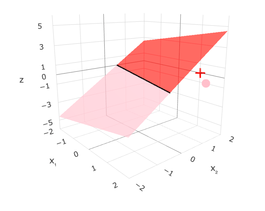
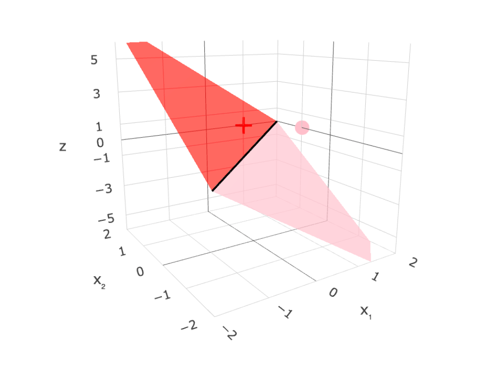
\({J}_{01}(\theta)\) is very hard to optimize (NP-hard) 🥺
- "Flat" almost everywhere (zero gradient \(\nabla_{\theta}{J}_{01}(\theta)\))
- "Jumps" elsewhere (no gradient)
linear binary classifier
features
parameters
linear combo
predict
\(x \in \mathbb{R}^d\)
\(\theta \in \mathbb{R}^d, \theta_0 \in \mathbb{R}\)
\(\theta^T x +\theta_0\)
\(=z\)
loss
linear regressor
- closed-form formula
- gradient descent
optimize
method
\(y \in \mathbb{R}\)
\(y \in \{0,1\}\)
training error almost "flat" w.r.t. \(\theta,\) so the gradient gives very little info
\(\mathcal{L}_{01}(g, y)\) is "flat" and discrete in \(g\)
\(g\) is "flat" and discrete in \(\theta\)
label
Outline
- Linear (binary) classifiers
-
Linear logistic (binary) classifiers
- to use: sigmoid
- to learn: negative log-likelihood loss
- Linear multi-class classifiers
linear binary classifier
features
parameters
linear combo
predict
\(x \in \mathbb{R}^d\)
\(\theta \in \mathbb{R}^d, \theta_0 \in \mathbb{R}\)
\(\theta^T x +\theta_0\)
\(=z\)
linear logistic binary classifier
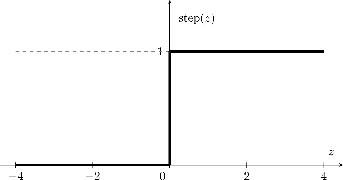
if \(z > 0\)
otherwise
\(1\)
\(0\)
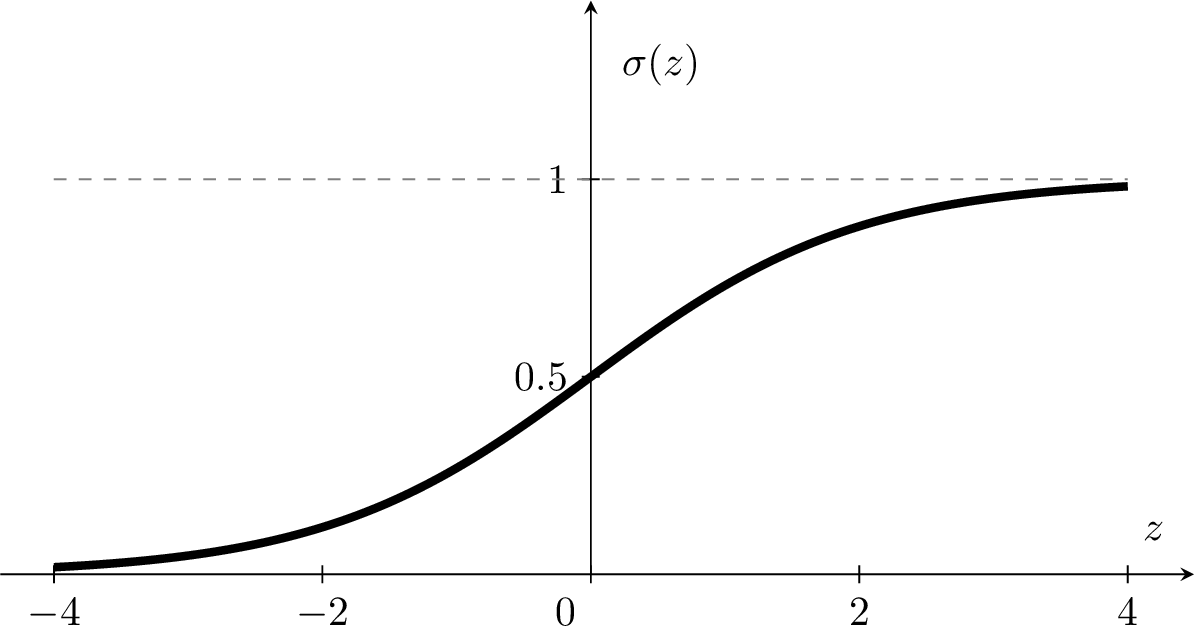
if \(\sigma(z) > 0.5\)
otherwise
\(1\)
\(0\)
\(\sigma(z)\): confidence, or estimated probability that \(x\) belongs to the positive class
label
\(y \in \{0,1\}\)
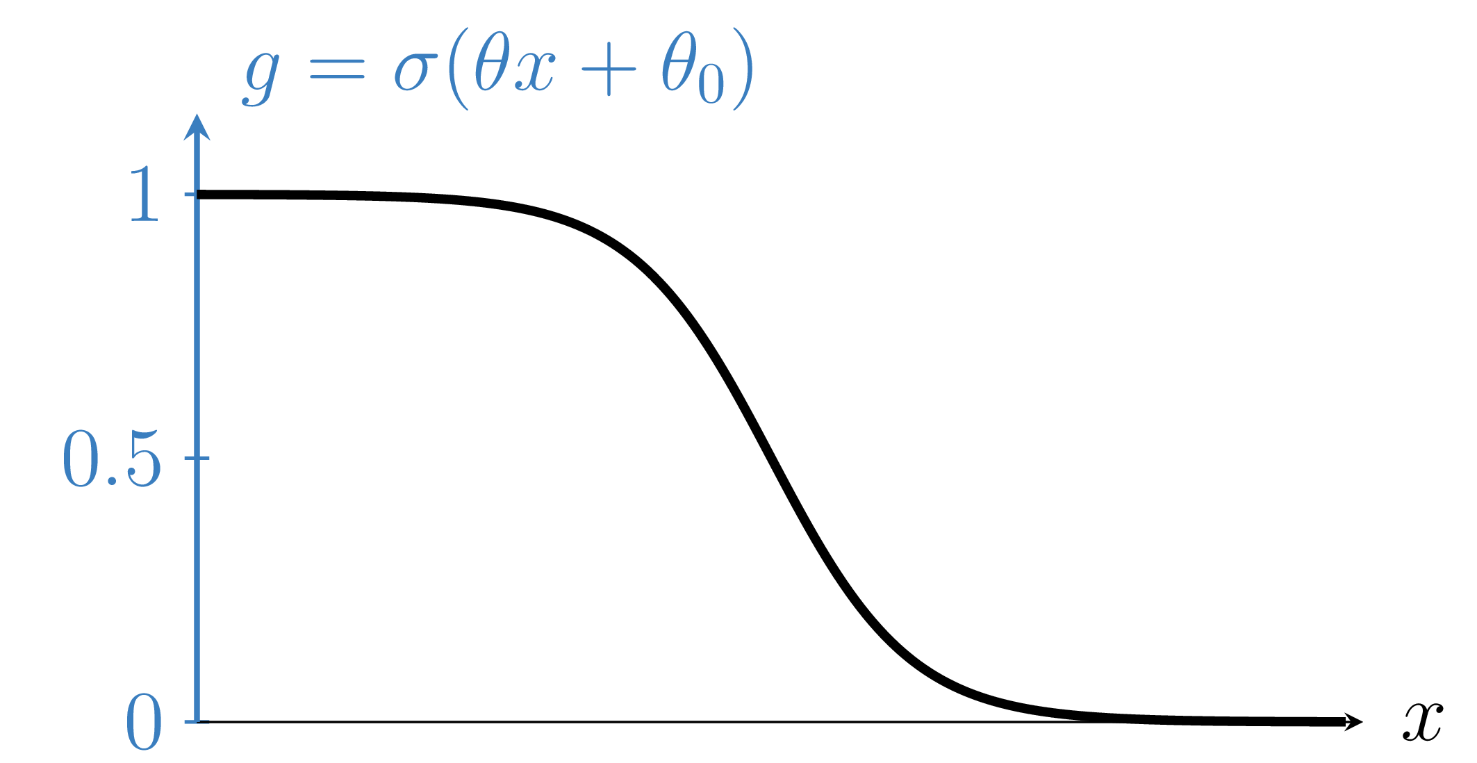
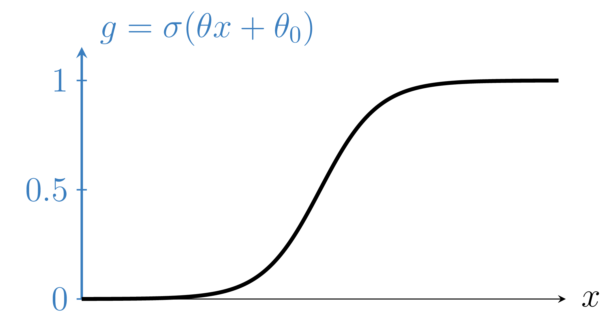
- \(\theta\), \(\theta_0\) can flip, squeeze, expand, or shift \(\sigma(\theta x + \theta_0)\) horizontally
- \(\sigma(z)\) is monotonic and has a tidy gradient (derived in hw/lab)
linear logistic binary classifier
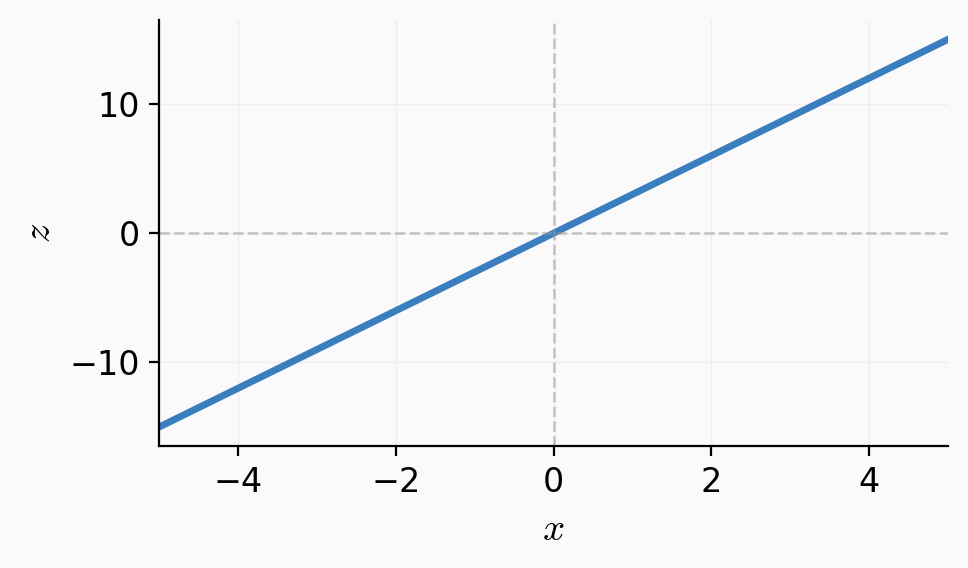
e.g., one feature
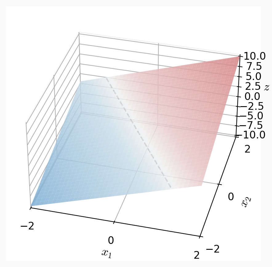
e.g., two features
features: \(x \in \mathbb{R}^d\)
parameters: \(\theta \in \mathbb{R}^d, \theta_0 \in \mathbb{R}\)
the logit \(z\):
apply sigmoid:
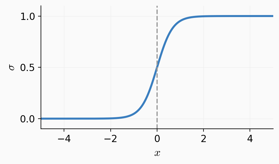
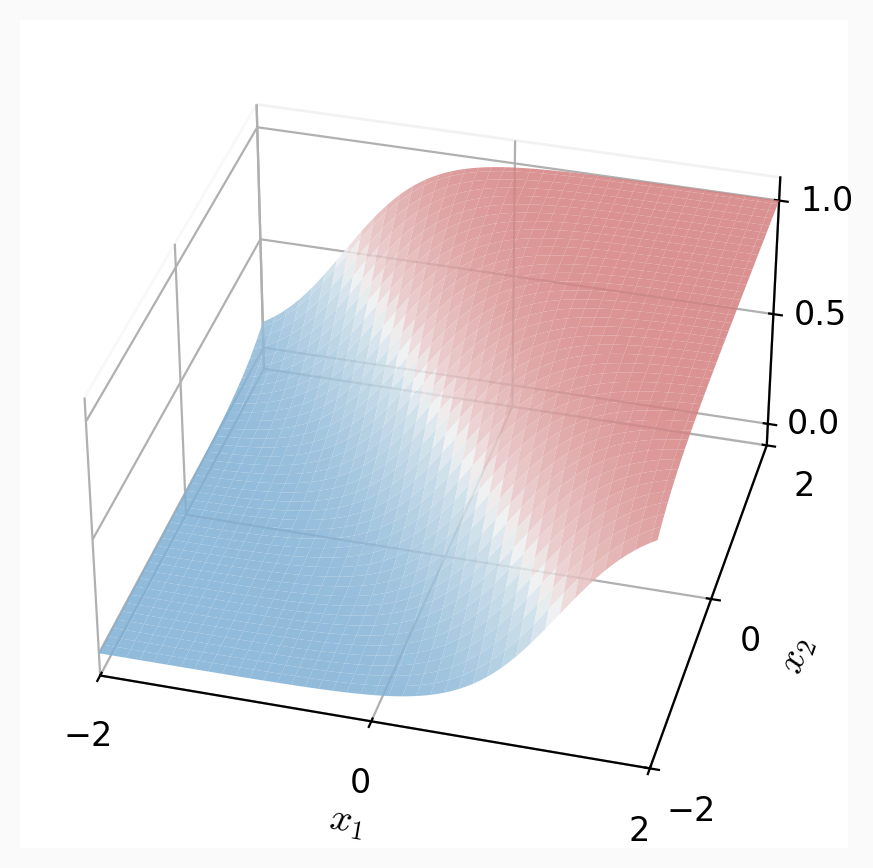
Predict 1 if \(\sigma(z) > 0.5\), else 0.
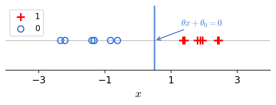
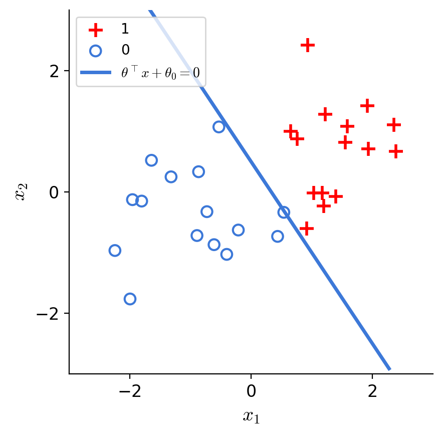
the separator is linear in \(x\)!
Outline
- Linear (binary) classifiers
- Linear logistic (binary) classifiers
- to use: sigmoid
- to learn: negative log-likelihood loss
- Linear multi-class classifiers
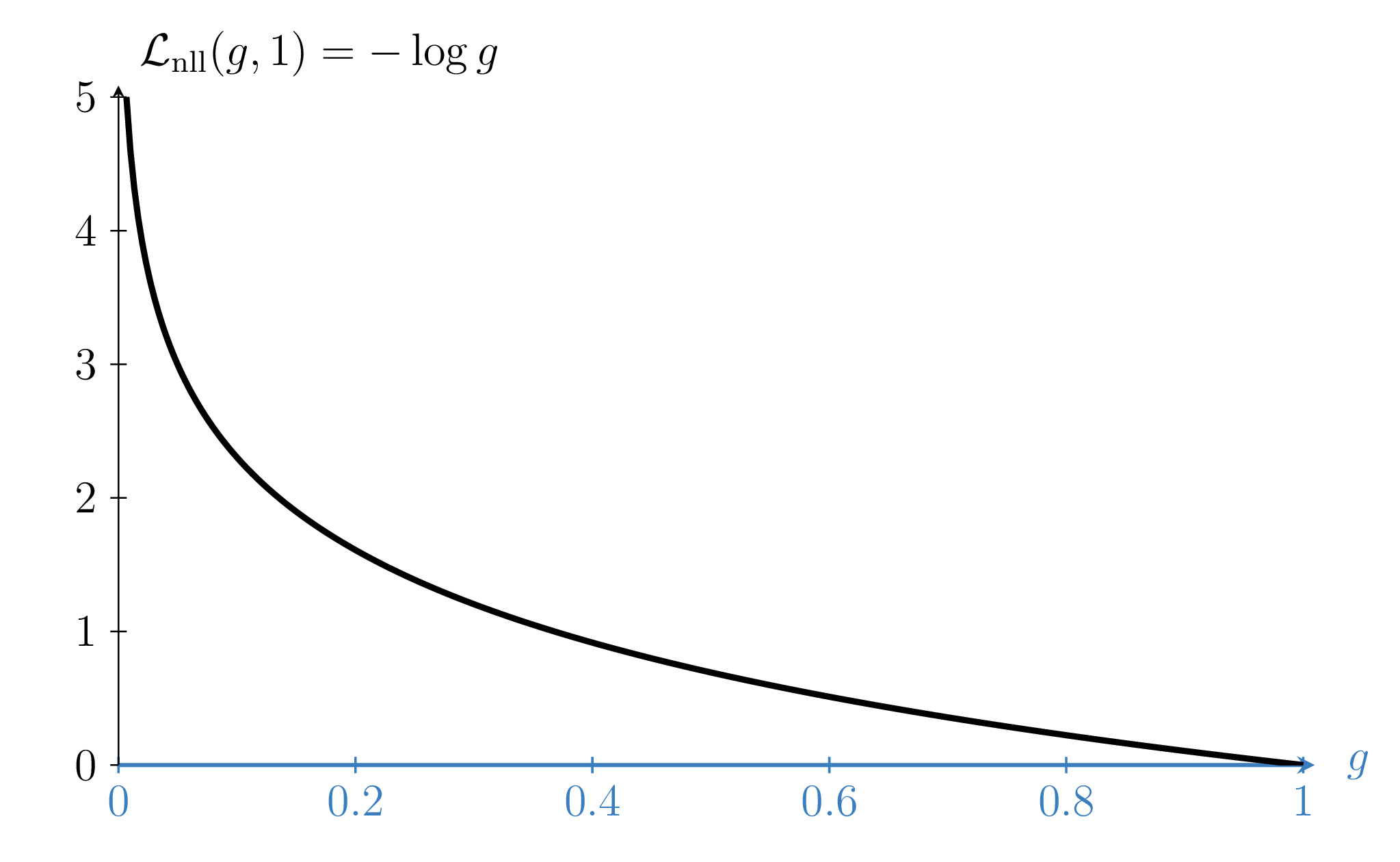
One training point, label \(y = 1\)
😍
🥺
😍
🥺

A smooth loss \(\mathcal{L}(g, y)\) that shrinks as \(g\) nears \(y\)?
negative
log
likelihood

😍
🥺
😍
🥺
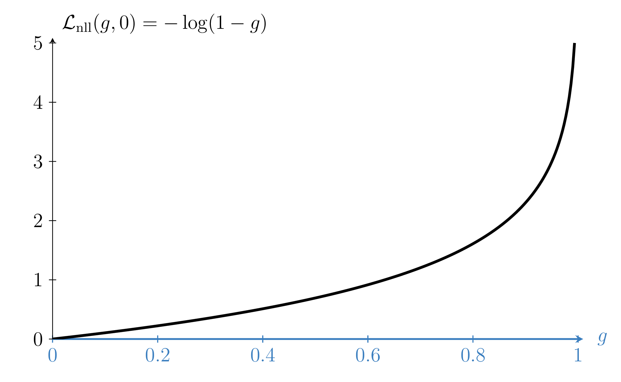
One training point, label \(y = 0\)
\(1-g\): the model's estimated probability that \(x\) belongs to the negative class.
Because the true label \(y\) is \(0\) or \(1\),
- When \(y = 1:\)
- When \(y = 0:\)
Read as: \(\sum\) (true label for class \(k\)) \(\cdot\) \(-\log\)(estimated probability of class \(k\)).
Since \(y \in \{0,1\}\), only the true class's term survives.
linear binary classifier
linear logistic binary classifier
features
label
parameters
linear combo
predict
loss
optimize via
\(x \in \mathbb{R}^d\)
\(y \in \{0,1\}\)
\(\theta \in \mathbb{R}^d, \theta_0 \in \mathbb{R}\)
\(\theta^T x +\theta_0 = z\)
no efficient method (NP-hard)
gradient descent
One training point, \(x = 1\), label \(y = 1\)
- If the data set is linearly separable, the logistic loss has no finite minimizing \(\theta\).
- In theory, \(\theta\) grows without bound, so the model gets overconfident.
- It is common to add a ridge penalty \(\lambda \|\theta\|^2\).
Outline
- Linear (binary) classifiers
- Linear logistic (binary) classifiers
-
Linear multi-class classifiers
- to use: softmax
- to learn: one-hot encoding, cross-entropy loss
Video edited from:
HBO: Silicon Valley, 2015.

ad (and graffiti) as seen on an MBTA train, 09/2026.
I'd say "Vibe code without the fundamentals"
🌭
\(x\)
\(\theta^T x +\theta_0\)
\(z \in \mathbb{R}\)
for two classes, {hotdog, not_hotdog}, one scalar logit \(z\) suffices
scalar logit,
raw score for hotdog
\(1-\sigma(z):\) estimated probability that \(x\) belongs to not_hotdog
\(\sigma(z):\) estimated probability that \(x\) belongs to hotdog
sigmoid
normalizing (squashing)
implicitly determines
for \(K > 2\) classes, one scalar \(z\) no longer suffices, so we use \(K\) logits, one per class
\(\theta \in \mathbb{R}^d, \theta_0 \in \mathbb{R}\)
🌭
\(x\)
\(\theta^T x +\theta_0\)
\(z \in \mathbb{R^3}\)
estimated probability that \(x\) belongs to hotdog
normalizing (squashing)
for \(K\) classes, use \(K\) logit scores.
e.g. \(K = 3\): \(\{\)hotdog, pizza, veggie\(\}\)
… to pizza
… to veggie
in general \(K\) logits
one raw score per class
\(\theta \in \mathbb{R}^{d \times K},\)
\(\theta_0 \in \mathbb{R}^{K}\)
outputs lie in \((0, 1)\) and sum to \(1\)
max among the \(K\) logits
"soft" max: the largest logit gets the largest probability
softmax: \(K\) logits to a distribution over \(K\) classes
e.g.,
sigmoid
predict the class with the largest softmax score
softmax:
predict positive if \(\sigma(z)>0.5 = \sigma(0)\)
unifying rule: predict the class with the largest logit (= largest softmax score)
implicit logit for the negative class
features
parameters
linear combo
predict
\(x \in \mathbb{R}^d\)
\(\theta \in \mathbb{R}^d, \theta_0 \in \mathbb{R}\)
\(\theta^T x +\theta_0\)
\(=z \in \mathbb{R}\)
linear logistic
binary classifier
one-out-of-\(K\) classifier
\(\theta \in \mathbb{R}^{d \times K},\)
\(=z \in \mathbb{R}^{K}\)
\(\theta^T x +\theta_0\)
predict positive if \(\sigma(z)>\sigma(0)\)
predict the class with the largest softmax score
\(\theta_0 \in \mathbb{R}^{K}\)
Outline
- Linear (binary) classifiers
- Linear logistic (binary) classifiers
-
Linear multi-class classifiers
- to use: softmax
- to learn: one-hot encoding, cross-entropy loss
One-hot encoding:
- Generalizes the binary labels \(\{0,1\}\)
Training data
| \(x\) | \(y\) | |||
| ( | 🌭 | , | "hotdog" | ) |
| ( | 🍕 | , | "pizza" | ) |
| ( | 🥗 | , | "veggie" | ) |
| ( | 🥦 | , | "veggie" | ) |
| \(\vdots\) | ||||
Training data
| \(x\) | \(y\) | |||
| ( | 🌭 | , | \(\begin{bmatrix}1\\0\\0\end{bmatrix}\) | ) |
| ( | 🍕 | , | \(\begin{bmatrix}0\\1\\0\end{bmatrix}\) | ) |
| ( | 🥗 | , | \(\begin{bmatrix}0\\0\\1\end{bmatrix}\) | ) |
| ( | 🥦 | , | \(\begin{bmatrix}0\\0\\1\end{bmatrix}\) | ) |
| \(\vdots\) | ||||
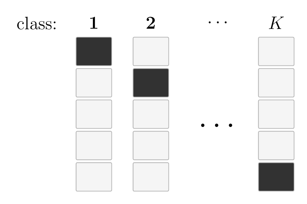
- Encodes the \(K\) classes as an \(\mathbb{R}^K\) vector, with a single one (hot) and zeros elsewhere
in general, for \(K\) classes:
- Generalizes the binary negative log-likelihood loss \[\mathcal{L}_{\mathrm{nll}}({g}, {y})= - \left[y \log g +\left(1-y \right) \log \left(1-g \right)\right]\]
-
Only the true class's term survives the \(K\)-term sum, since every other \(y_k=0\)
Negative log-likelihood multi-class loss (also called cross-entropy)
\(y:\) one-hot encoding label
\(y_{{k}}:\) \(k\)th entry in \(y\), either 0 or 1
\(g:\) softmax output
\(g_{{k}}:\) estimated probability that \(x\) belongs to class \(k\)
🌭
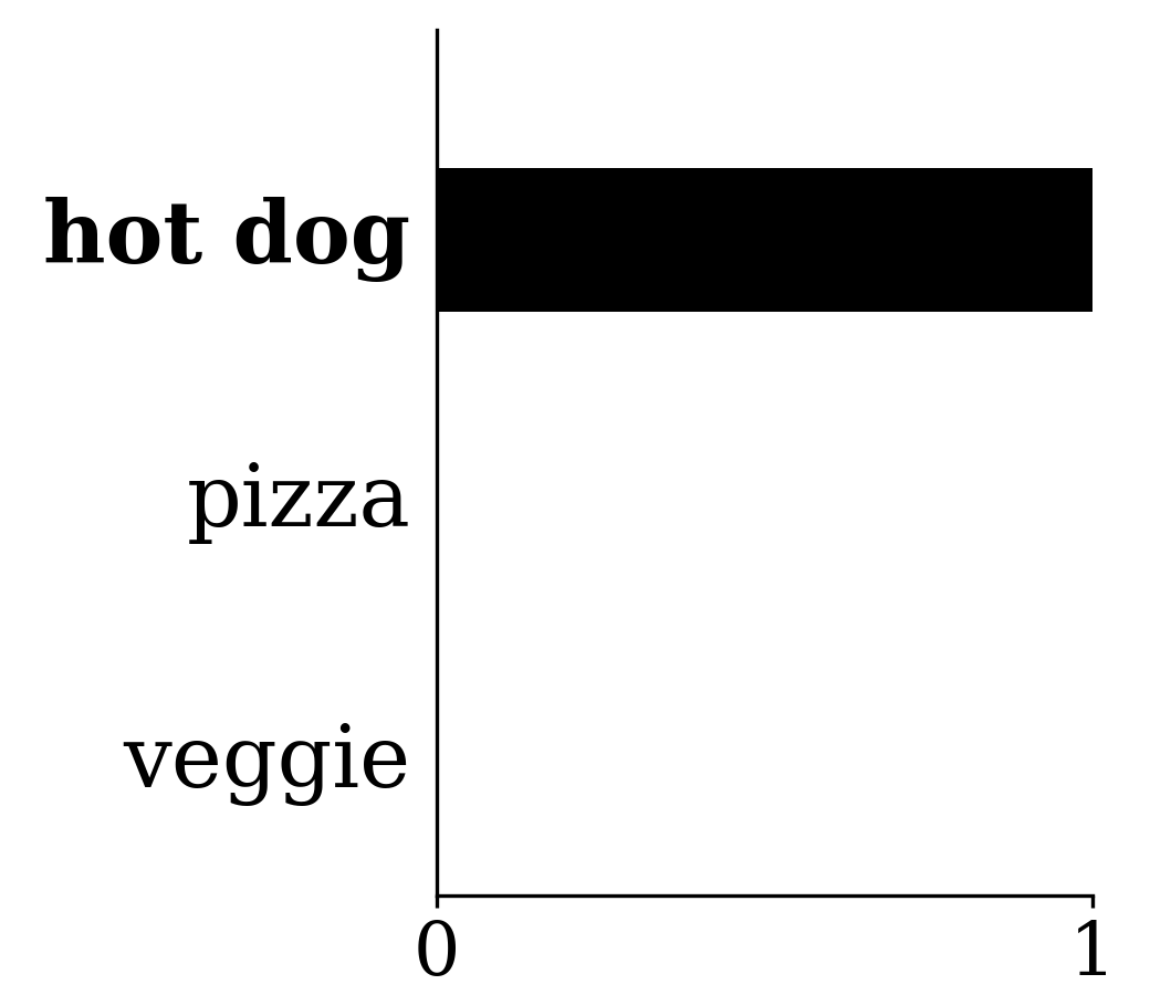
current prediction \(g=\text{softmax}(z)\)
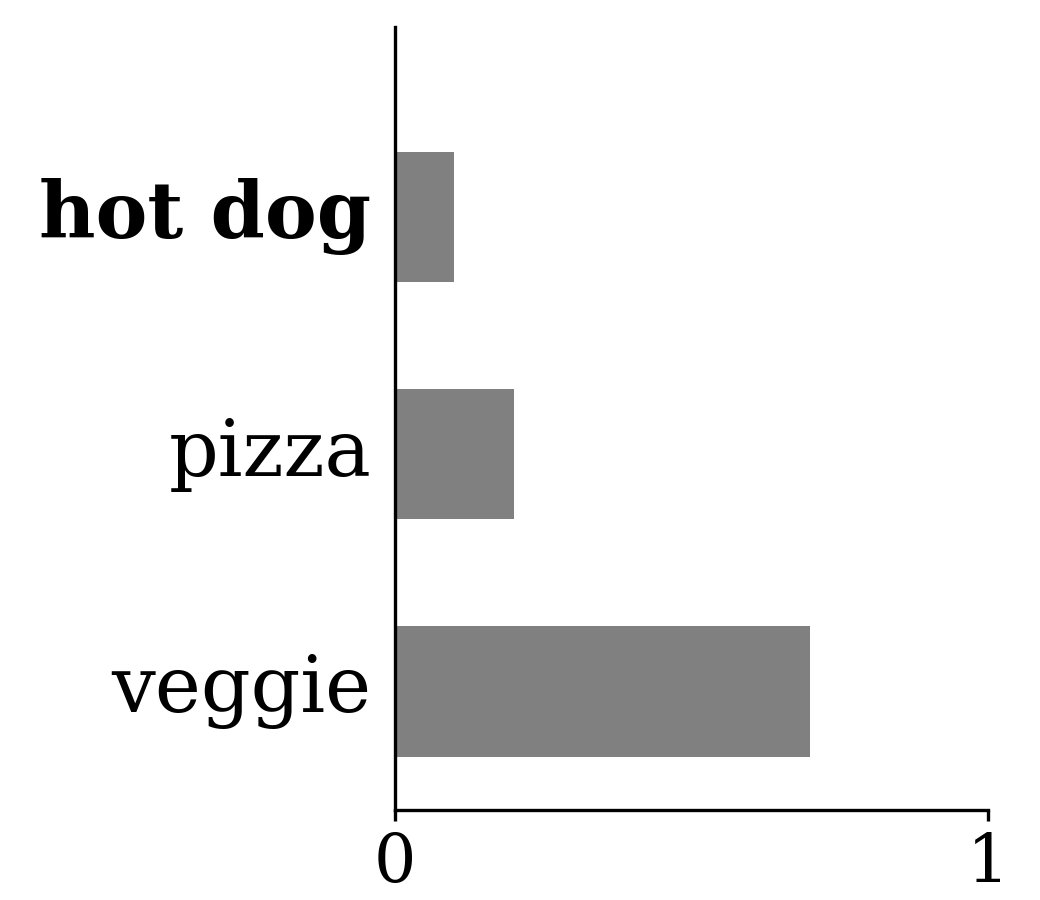
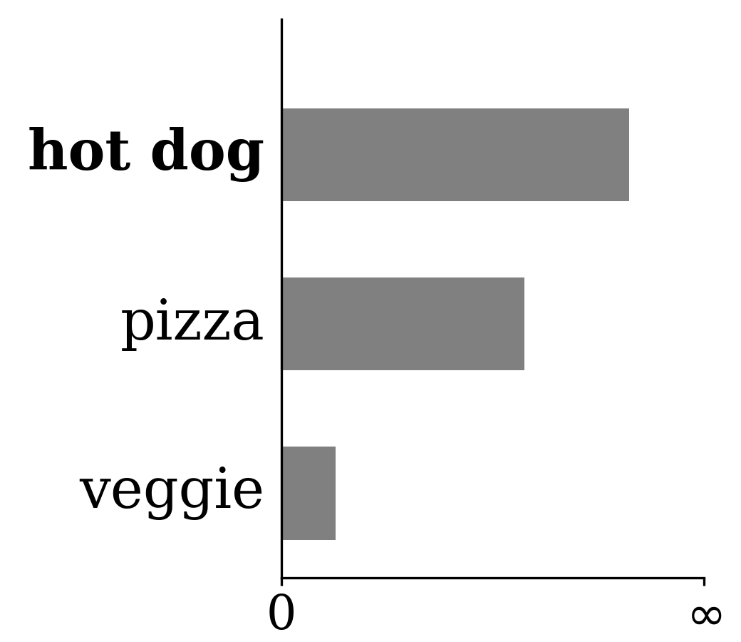
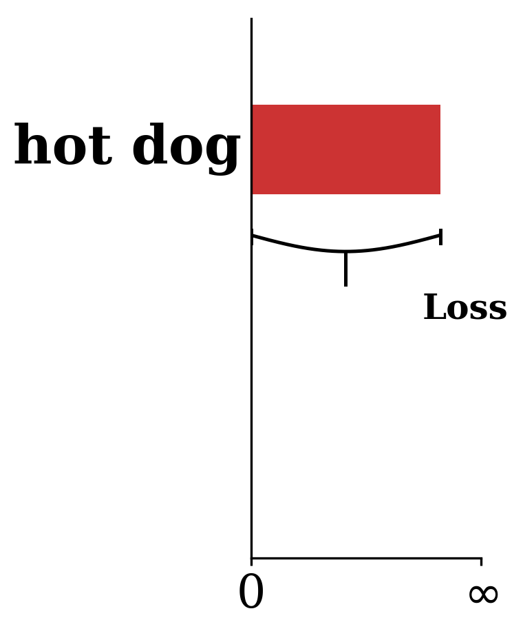
end-to-end pipeline
contrived predictions
To reduce the loss, \(g_{\text{hotdog}}\) needs to go up.
That signal flows smoothly back to \(\theta\) through \(-\!\log\) and softmax, so gradient descent can train \(\theta\).
🌭
current prediction \(g=\text{softmax}(z)\)
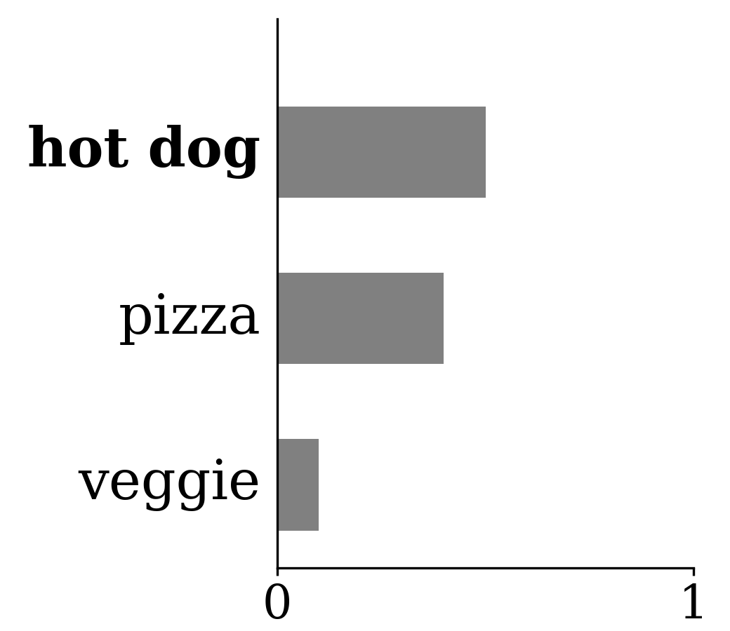
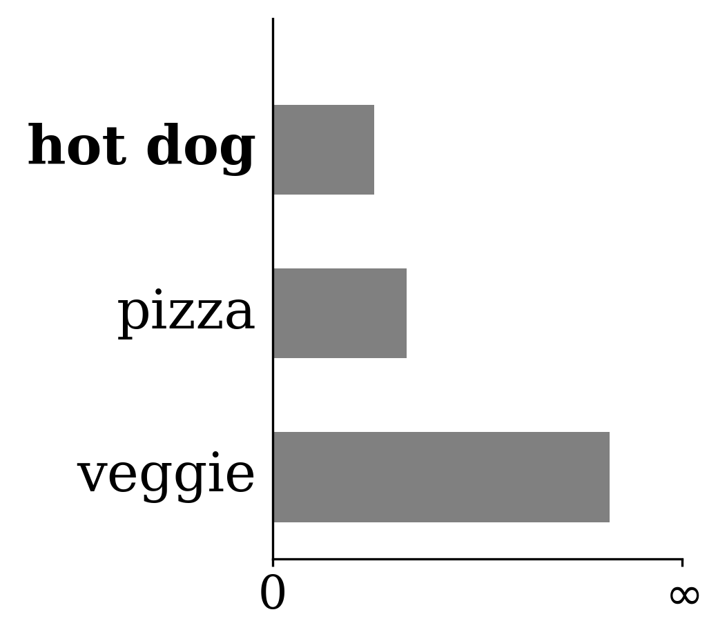
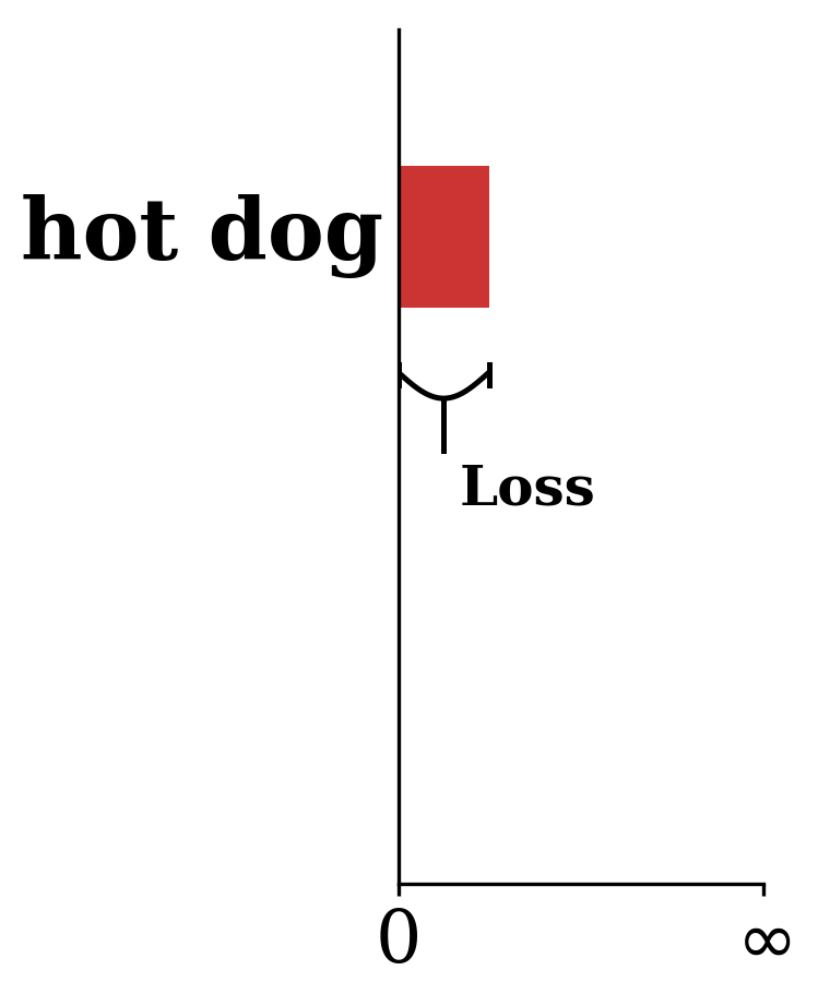
end-to-end pipeline
contrived predictions
Summary
Linear (binary) classifiers
separatornormal vector0-1 loss
Linear logistic (binary) classifiers
sigmoidlogitnegative log-likelihoodlinearly separable
Linear multi-class classifiers
softmaxone-hot encodingcross-entropy
\(\mathcal{L}_{\text{nll}}(g, y) = -\left[y \log g + (1-y) \log (1-g)\right], \quad g = \sigma(\theta^T x + \theta_0)\)
-
Linear (binary) classifiers
to use: predict 1 when \(z = \theta^T x + \theta_0 > 0\); the separator \(z = 0\) is a hyperplane with normal \(\theta\).
to learn: the 0-1 loss is flat in \(\theta\), so there is no gradient to follow.
-
Linear logistic (binary) classifiers
to use: \(g = \sigma(z)\) is a probability, and \(g > 0.5\) exactly when \(z > 0\), so the separator stays linear.
to learn: the negative log-likelihood is smooth, so gradient descent works; on separable data, a ridge penalty keeps \(\theta\) finite.
-
Linear multi-class classifiers
to use: softmax turns one score per class into a distribution; sigmoid is its two-class case.
to learn: one-hot labels and the cross-entropy loss, \(-\log\) of the true class's probability.